The sound of chaos
What is chaos?
Chaos is a concept related to dynamical systems, that are nothing but systems than can be described by amounts that change in time. There are examples of dynamical systems everywhere: the amount of money in your bank account, your weight, your room’s temperature, … all of them evolve in time, and therefore are dynamical. The electromagnetic field, chemical concentration of a reactive, population of a species, position of an object, … are also good examples1.
The natural language for dealing with dynamical systems is that of difference and differential equations. For example, if I’m adding 1 cent every day to my bank account, my amount of money (x) will grow as:
x(today) = x(yesterday) + 1 cent
Or, if my acceleration is constant (as happens in free fall), my speed (v) will evolve as:
![]()
Both of them have in common that, knowing the state of the system at a given time, they provide an update rule to compute the state in the future, i.e., are deterministic equations.
The variety of behaviors in dynamical systems is as broad as its enormous range of applicability, but most of them can be classified in one of these three categories by looking at their long-term behavior:
- Stable systems: the variables tend to a fixed value, like, for example, the temperature of a boiling pot (that stabilizes at ~100ºC). In this case, a plot of the variable shows clearly that the variable starts moving slower and slower until it virtually stops.
- Unbounded unstable systems: the variables keep growing (or decreasing) indefinitely, like, for example, in an ideal savings account with no withdrawals. If we plot the variable against time, we will find that the variable never stops moving away and away.
- Cyclic unstable systems: the variables tend to a periodical behavior, like, for example, the voltage of certain electric circuits. As in the previous case, the variable never stops moving, but it will move cyclically without never going too far away.
But there is another, more bizarre, possibility: chaotic systems. Indeed, chaos is so strange that the easier way to define it is in negative terms. Chaos is not contained in any of the previous categories, so it is unstable, bounded and not cyclic.
One of the first difficulties for getting an intuitive idea of chaos is that we need at least 3 dimensions to find chaotic behavior (at least is not 4!). We can picture a three-dimensional variable using the movement of a fly inside a room as an analogy. The distance to three different walls reads as the three elements of the variable (x(t), y(t), z(t)). So, going back to our three “easy” categories:
- A stable fly will fly slower and slower until virtually stopping.
- An unbounded unstable fly will fly away to infinity.
- A cyclic fly will fly in a closed curve again and again.
What about a chaotic fly? Can we picture its movement? Yes, we can! A chaotic fly will fly following the trajectory of a strange attractor. Below you can see an example of one of these attractors, known as Lorenz attractor:
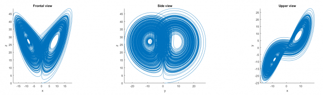
The trajectory of our imaginary fly has some outstanding features: it is confined inside a small subset of space (you can build a box for it, and it will fit inside), and despite it never stops advancing (so its length becomes larger and larger), the curve never crosses nor closes itself2. Think about it, this is a pretty bizarre geometry. Indeed, those attractors are fractal structures.
Another remarkable property of chaotic systems is its long-term unpredictability. If we run the same chaotic dynamics with only a very small difference at the starting point, both trajectories will soon diverge until they reach a saturation distance, comparable to the size of the bounded region where the attractor “lives”.
One may think that the arising of chaos requires very complex dynamical rules, but surprisingly this is not the case. Indeed, lots of natural phenomena are chaotic, ranging from population dynamics in ecology1 to geomagnetic shifts 2.
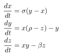
The classical example of the Lorenz attractor is just the result of a three-dimensional ordinary differential equation that appears in climate modelling, and even in the mechanics of a water wheel. It doesn’t look very scary:
The sound of chaos
If we look at each coordinate (x, y, z) separately we will find three noisy looking time series:
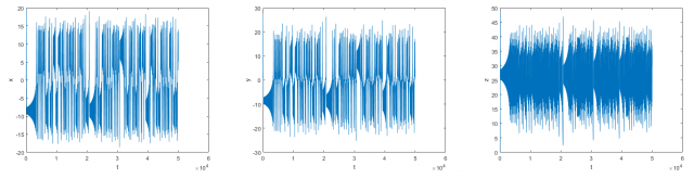
So, what happens if we send one of this time series to our speakers?
First of all, we have to think about the process of sonification of a signal, that is, transforming our time series to an audible audio signal. For being able to accomplish this we’ll need to:
- Perform the small conceptual leap of thinking of the signal intensity as a mechanical vibration. If you think about it, this is not different to understanding the signal intensity as height in a graph.
- Extract a one-dimensional time series. In our case, we picked separate cartesian coordinates, but it is important to note that this is an arbitrary choice
- Normalize the signal between -1 and 1.
- Modify the frequency signal to fit it into the auditory range of human beings (~20 – 20.000 Hz). This is done just adjusting the speed we use to read it… the faster, the higher the frequencies.
You can hear the results in the following links:
It sounds like noise, but it is not. It is deterministic chaos!, way cooler than noise!
If you want to experiment yourself, you can download the Matlab script I’ve used to solve the Lorenz problem and generate this audio file using this link.
An unexpected application
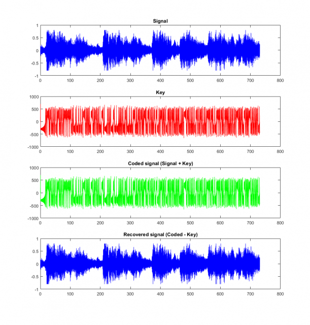
The almost total absence of structure in chaotic “noise” can be used in a straightforward way to send secret messages.
For doing so, one can just add a loud chaotic signal to an audio signal, so the result will be completely unintelligible. This information can be safely sent to a receiver who, knowing before the same chaotic time series, can subtract it to the original signal and so, decode it.
A Matlab script doing exactly this to encrypt an excerpt of Handel’s Hallelujah can be downloaded using this link.
Remarkably, some electronic devices can reproduce the behavior of a given chaotic system3, and have been used as emitters and receivers that automatically encrypt the message3.
Notes:
1The latter one, position, is especially relevant because a whole branch of physics, mechanics, is devoted to the time changes of position, better known as movement.
2This is the main reason for the impossibility of chaos in two dimensions. The curve has not enough free space to evolve without crossing nor closing without falling into one of the three non-chaotic categories.
3There are some fascinating details about the synchronization of both emitter and receiver that are beyond the scope of this article. For more information, see (Strogatz, 1994)
References
- Scheffer, M., & Carpenter, S. R. (2003). Catastrophic regime shifts in ecosystems: Linking theory to observation. Trends in Ecology and Evolution, 18(12), 648–656. doi: 10.1016/j.tree.2003.09.002 ↩
- Pétrélis, F., & Fauve, S. (2008). Chaotic dynamics of the magnetic field generated by dynamo action in a turbulent flow. Journal of Physics: Condensed Matter, 20(49), 494203.doi: 10.1088/0953-8984/20/49/494203 ↩
- Strogatz, S. H. (1994). Nonlinear Dynamics And Chaos: With Applications To Physics, Biology, Chemistry And Engineering. Perseus Books Publishing. ↩
6 comments
Really cool article, thank you. I do know know much about math, but I have this question: if chaos is not “cyclic” how come that the figures you showed above form some kind of closed curves? Would that not make them cyclic in a mathematical sense? Cyclic = relating to a circle or other closed curve.
Hi Il postino, thank you for your comment and your question.
The reason why the curves look closed is just a matter of visualization. All them are a 2D projection of a 3D object, so a piece of curve passing behind another one look like a contact (but it is not).
On the other hand, the curves wind closer and closer, so the resolution is never good enough! Anyway, if you zoom on the Matlab figures (you can download the code here) you’ll see that indeed they don’t collide.
For more details about the question about the colliding or not of the phase curves, I suggest reference 3 (Strogatz, 1994).
Thank you for your kind response.
[…] Para obtener una idea intuitiva de lo que es el caos podemos visualizarlo o escucharlo. Pablo Rodríguez-Sánchez nos dice cómo en The sound of chaos […]
Well written, are you a science writer as well. We are really in demand of good communication about nonlinear systems / ecological systems and many more. Not at least under the sustainability demands. Itwould be nice to hear more from you.
Hi Michael, and sorry for the late reply. For some reason, this webpage doesn’t send notifications about new messages.
Feel free to take a look at my portfolio: https://pabrod.github.io/pages/portfolio-en.html
Cheers!