Behaviour and genes: burrowing and loci.

How are we like we are? What defines our mind, our character, and our behaviour? Men made ​​themselves these questions in all ages of humanity. From the age of myths to the age of science the answers have been very many. We do not have an adequate answer yet, maybe never. However, the rise of Genetics, Biochemistry and non-invasive techniques is sharpening the methods of the behavioural sciences to suggest a combined and complex gene-environment action in modulating the behaviour of living beings. Nowadays, addressing high complexity studies where many factors come into play is becoming more feasible due to the fact that new technologies make easy to find patterns otherwise neglected by our eyes. In any case, to find simple examples of the relationships between genes and conducts will help us to understand solidly the bases of the behaviour underlying processes.

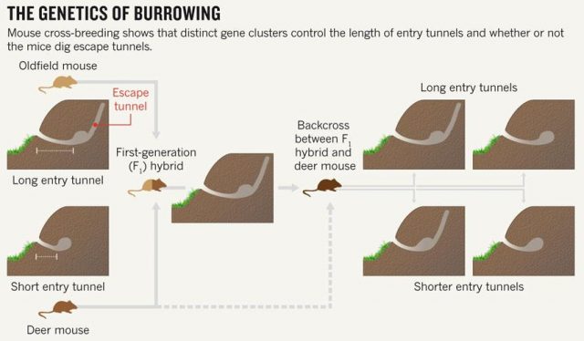
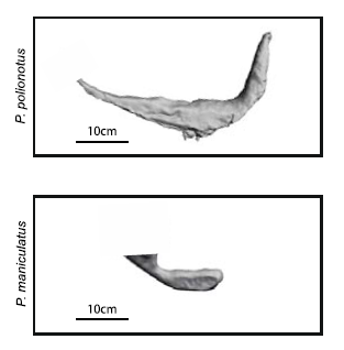
Studying animal behaviour is been for long a really interesting field. It has brought important findings about evolutionary traits of animal actions. But, how can we measure de animal behaviour? There are several answers, but a good option is to consider animal architectures. Nests, spider webs or burrows have parameters that are more or less easy to measure and, most likely, have emerged and evolved due to natural selection. Therefore, to establish the connection between animal architecture parameters and certain genes can help considerably in understanding the relationship between genes and behaviour. That’s what they do in this paper Weber and co-workers ¹. They explore the relationship in between some genetic modules of two close mouse species and their different behaviour digging their lairs. One of them, P. polionotus, construct burrows with a long entrance ended in the nest cavity. The nest, in its backside, has a secondary not-opened tunnel that terminates just below the soil surface. The other, P. maniculatus, drills just small simple burrows with only a single entrance tunnel (Fig. 1).

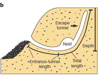
Apart of making different kinds of burrows, these two mouse species have different habitats and geographic distribution. While P. polionotus is an open-field (beach and old fields) specialist limited to southeastern United States, P. maniculatus is generalist from North American forests and grasslands. Here, the former could use the secondary tunnel as escape route when predators attack the main entry in such an open area. But the differences in burrowing of this two species could be also due to the differences in the ground composition and hardness. To rule out which characteristics of the burrow were depending on the soil type they studied natural P. polionotus constructions. It was found that shape and length were conserved while burrow depth was affected by soil composition. Hence, they studied the burrowing behaviour using the entrance length and shape (presence of scape tunnel) of the burrows of both, P. polionotus and P. maniculatus, and also their first-generation hybrids (F1) and recombinant backcrosses (BC, that is F1 animals with P. maniculatus) in laboratory controlled conditions. Worth to say that the burrowing experiments were done with mice bred in captivity and exposed to make borrows never before. So their burrowing behaviour, which finally resulted similar to their wild peers, was not learned but having a strong genetic component.

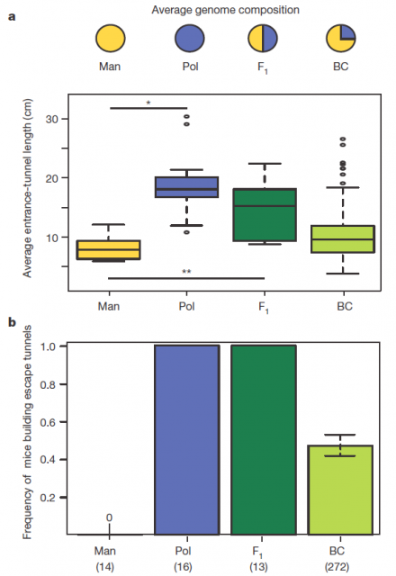
Figure 2 summarizes some interesting observations: having a genetic composition that is half of each parental line F1 burrowing behaviour is more similar to P. polionotus, building burrows with long entrance tunnel and also escape tunnel. This means that the alleles¹ involved in burrow size and shape would show dominant segregation. But often things are not that simple. The recombinant backcrosses, which have a genetic composition that is three quarters of P. polionotus, display a continuous gradient of entrance length between parental extremes and scape tunnel only in half of the population. Therefore in one side, the entrance-tunnel length could depend only in few loci^2. In the other side, building scape tunnel could be produced by a single locus³ or also by a multi loci interaction with a threshold effect⁴.

Consequently, these differences into the inheritance of those two traits point out to two separate behavioural modules. In order to identify the genomic regions affecting these mice´s digging behaviour, they used a technic named Quantitative trait locus (QTL) mapping⁵. By analysing the F1 hybrids, four genomic regions (or linkage groups⁶ to be more precise), each in different chromosome, were found contributing to those two modules. Three of them in the chromosomes 1, 2 and 20 were involved in entrance-tunnel length. The other in chromosome 5 was associated with presence of escape tunnel.

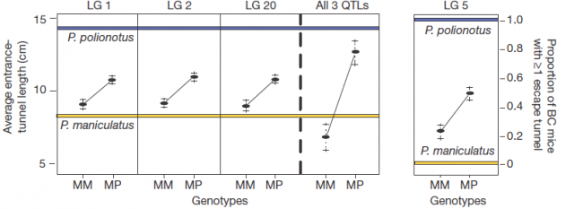
Afterwards, comparing the burrowing behaviour and genotypes in BC mice, they found that P. polionotus alleles were dominant for the entrance length but not for constructing escape tunnel. Those BC mice heterozigotes (MP) for the linkage groups in chromosomes 1, 2 and 20 displayed almost the same entrance-tunnel length than F1, while BC mice homozigotes (MM) were quite similar to P. maniculatus (Fig. 3 left). Therefore, the continuous tunnel-length variation observed in BC mice could be explained by the inheritance of only few genes located in those linkage groups. Depending on the allelic composition, which varies between the two extremes (from 6 alleles M to 6 alleles P), the entrance of the burrow would range from shorter to longer. In relation with the escape tunnel, BC mice heterozigotes (MP) built the secondary tunnel with 50% probability. However, homozigotes (MM) did the same with 20% probability even when P. maniculatus, having that same theoretical genotype for that trait, never makes escape tunnel (Fig. 3 rigth). For this reason, the genomic region (in chromosome 5) isolated by QTL is insufficient to explain the observed variation in construct escape tunnel, either because inadequate markers for this trait were used in the QTL or because the loci involved in it are additive or epistatic⁷. Whatever the reason for not finding the complete set of genes involved in this module of behavior (QTL has its limitations), it seems that the construction of escape tunnel evolved independently of the entrance length. Going a bit beyond it could said that P. polionotus complex digging behaviour emerges upon interaction between simple behaviours that could appear with different gene clusters.

Pretty nice example above to illustrate the approach between behavior and genes. Not perfectly delimited, it´s being for quite a while that things are no longer black or white in genetics. Either way, to find out and to prove that few genes are able to explain a behavioural trait, as if it were a morphological character, says much about the physical bases of something considered as ethereal as the way of being. Some studies as the present one are beginning to show substantial evidence of how some genes or groups of them modulate certain behaviors. In this case implies that part of the behavior is innate, at least in mice. Others claim that long-term mice memory, and therefore learning, depends largely on chromatin regultion by histone acetyl transferases (for Review: S.C. McQuown, M.A. Wood/ Neurobiology of Learning and Memory 96 (2011) 27–34). What if you think about, it is just another stone in favor of genes controling behaviour. It´s still quite early to make balance, it is known that genes respond to the environment, but ultimately, the answer depends on the gen or allele which is available. Therefore, though our behavior is quite far from the rodents and the cultural components are quite heavy in primates, to elucidate the molecular mechanisms controling the behavioural processes may help to understand ourselves and more important, to face any sort of mental disorders. My hope would be to see here something like what happened when deep study of simple monogenic diseases laid the foundation for understanding diseases with more complex genetic causes.

Explanatory notes

1) Allele: each of the variants of the same gene.

2) Loci: plural for Locus

3) Locus: position within a chromosome where a gene, a marker or determined DNA sequence is located physically.

4) Threshold effect: here, a visible effect is shown only when several loci interact exceeding certain quantitative limit.

5) Quantitative trait locus (QTL): This is a method of statistical analysis that uses trait measurements and genotypic data to explain the genetic basis of variation in complex traits. After crossing different strains of a given organism, the genome of their hybrids is analysed looking for segregation frequencies of genetic markers like SNPs (single nucleotide polymorphisms). Markers that are physically close to the locus or loci that modulate the trait of interest will segregate with frequencies more similar to the frequency of the trait. However, unrelated markers will segregate without significant association with the trait. (Source: Miles, C. & Wayne, M. (2008) Quantitative trait locus (QTL) analysis. Nature Education 1(1):208).

6) Linkage group: it is a set of genes or genomic sequences inherited together due to their close proximity within a chromosome region. As closer they are, less probable it will be that they recombine between chromatids during meiosis. Therefore, the alleles of such a set of genes will be inherited together with high probability.

7) Epistasis: when a trait emerges from the interaction between different genes.