Waning planets: the smallest planet ever detected

The Kepler mission is gazing at the Universe. Every little twinkle in more than 150,000 stars is being recorded since 2009, looking for planetary transits. And this will continue for at least three more years, giving us insight into the wondrous nature of the planetary systems in our galaxy’s vicinity. So far, we had witnessed giants crossing in front of stars and became familiar with concepts such as hot-jupiters, super-terrae and so on. But, what lies in the opposite side of the spectrum?

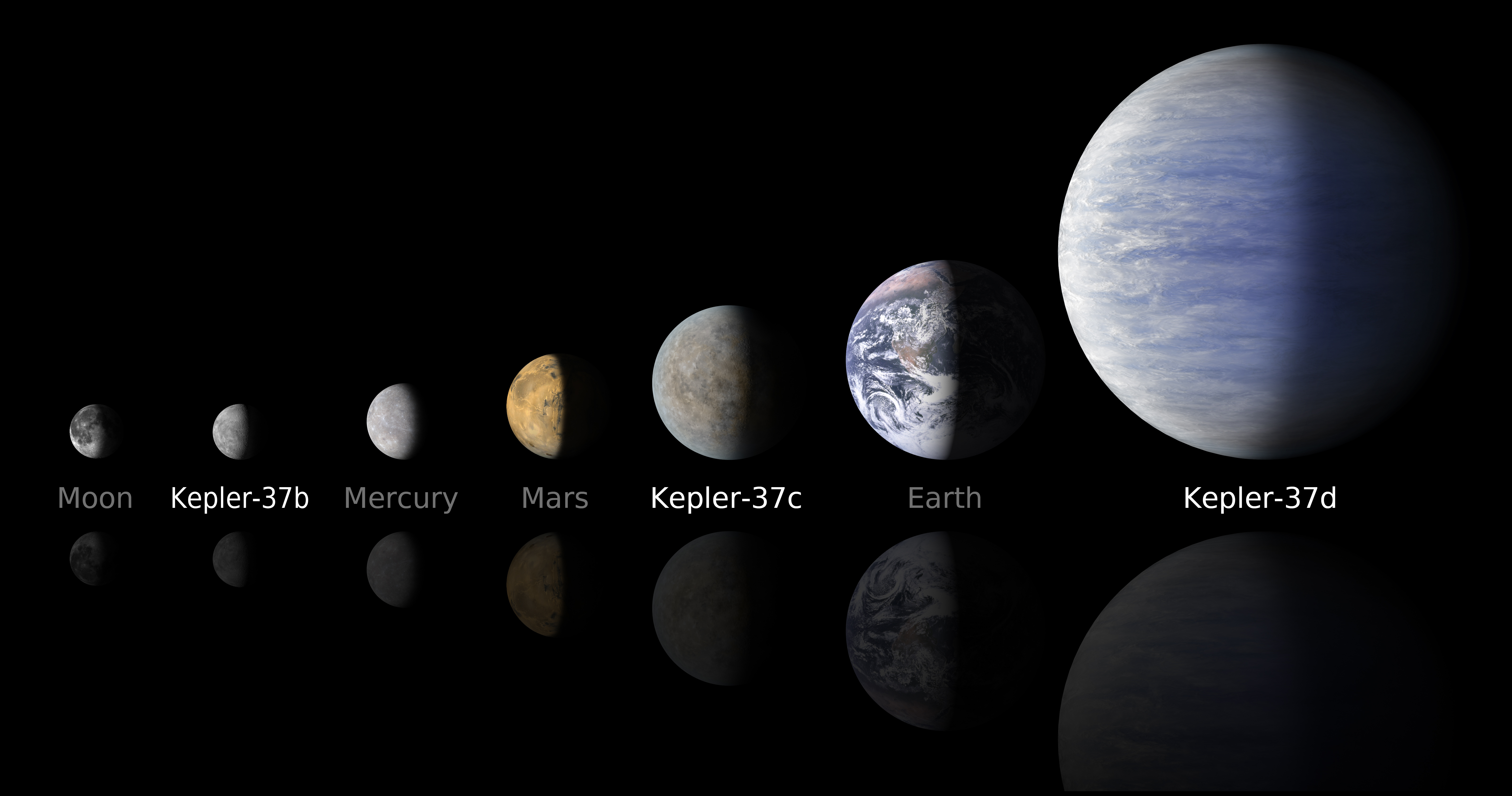
This question has been addressed by Barclay and collaborators in a paper recently published by Nature magazine ¹. Their work shows that star Kepler 37 hosts the smallest planet we have ever seen, even if we include Mercury in our own Solar System. Such a tiny planet is called Kepler 37b and it is not alone. Two other planets orbit farther around the star. They are probably somewhat between Mars and the Earth in size (Kepler 37c) and twice as big as our pale blue dot (Kepler 37d). However, Kepler 37b really makes the difference: being just slightly larger than the Moon it is not only a technical challenge for detection but it is also a first step towards understanding how common small planets can be.

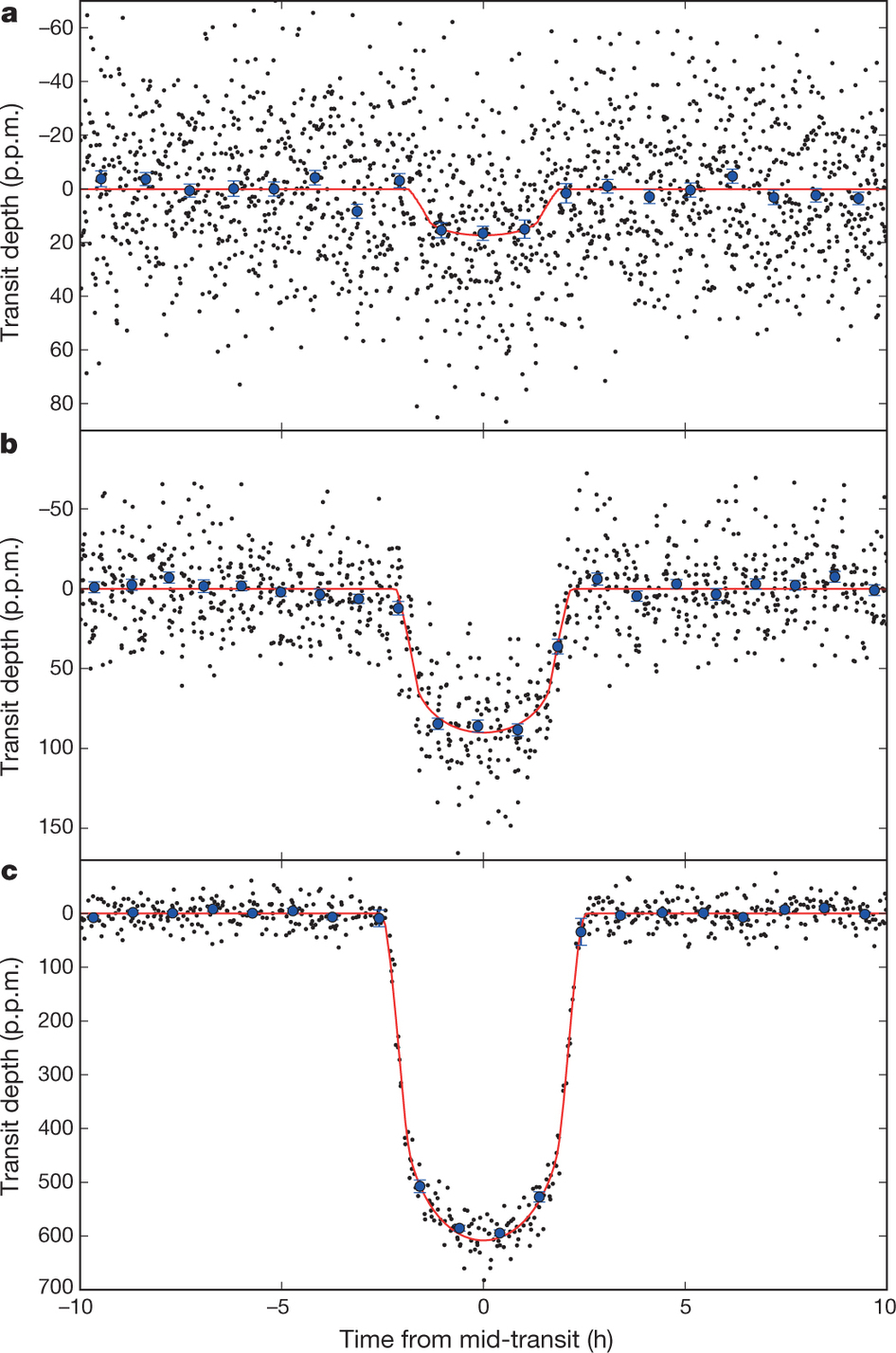
The idea that supports the detection of planets by means of planetary transits is pretty straightforward ². If you happen to find a planet crossing in front of its star from your point of view (‘a transit’), you could in principle detect a decrease in the amount of light reaching to your telescope. The first problem is that such a decrease of incoming flux is small enough to get lost in our measurements noise. Increasingly efficient detectors and, more importantly, moving our observatories to space has allowed the detection of almost 300 planets using this technique, as of February 2013 ³.

However, there is still a second, more subtle problem. How can we discriminate between false positives and real planets? This is not an easy question to answer. What kind of artifacts can contaminate our detections? All stars show an intrinsic variability up to a certain extent, related to their mass and temperature. This is commonly assumed to be well determined by the models of the interior of stars. In short, cold stars use to show more variability than hot stars. This point is central for the studies developed by the Kepler mission. Let’s assume we can get rid of this kind of problems by observing some well-behaved stars.

Even if we are observing the perfect star, the photometric aperture of any instrument needs to be big enough to get a good signal to noise ratio. Kepler mission’s aperture is, for example, some arc seconds across. This also increase the chance of inadvertently including any other star in the measurements, something which is usually termed a ‘blend’. It wouldn’t be a problem if this is a lonely star, it would just increase the incoming flux without any other side effect. However, the star could be orbiting the very same planetary system we try to detect, in what is called a ‘hieararchical triple’. In this case, the foreground or background star would add a periodic effect that could mimic a planetary transit, leading us to error. Another type of blend that could fool us is having a binary system inside our photometric field. This would, again, introduce a periodic signal potentially raising a false positive.

There are, of course, a number of sanity checks for avoiding those situations. The rule of the thumb is ‘get as many observations as you can’. If you are able to get spectroscopy from your photometric candidates then you are very likely to success. Unfortunately, spectroscopy of faint pairs is very expensive in terms of telescope time and therefore not always feasible. Other methods for avoiding false negatives include checking the depth of secondary eclipses, trying to determine changes in the centroid positions correlated with the brightness changes, detect transit timing variations (TTS) and many others.

Suppose that we still have a candidate not suitable for this sort of verifications, what can we do? Guillermo Torres, one the co-authors of the paper, and his team at Harvard University developed in 2004 a code called BLENDER in order to compute the chance that our observations of a given system are contaminated by ‘blends’ ⁴. Instead of trying to demonstrate that we have a planet, let’s work on the opposite hypothesis: what we see is just a blend with a field star. Restricting ourselves to the two blend categories we have already described, the code will generate a hieararchical triple or a background binary and try to fit data. The free parameters of the problem are the mass of the star, distance, inclination angle and so on. There are a number of constraints to the blend due to the fact that members of a multiple systems usually have the same age (they are said to be in the same isochrone) and so stellar interior models put a limit to their possible properties. If we scan the free parameter space with a grid of possible models we can find which of them are elegible for reproducing our observed light curve. If the blend happens to reproduce well the observed variation of the incoming flux, then the model is assumed to be very likely. Conversely, if the fits are poor, then the blends are unlikely and we can be quite sure that our planetary system is real.

This is what Barclay et al. did for Kepler 37 system. They find that there is just one chance in a million that the biggest planet (Kepler 37d) is an artifact. The odds ratio in favour of the second planet, Kepler 37c, is 287 and 262 for the smallest one, Kepler 37d. However, if we include co-planarity in the system (something which is expected, in fact), chances get up to 99,95% that both planets are real. And this opens a full new range of planets out in the Universe. This could be the first planet of the most common family in the Galaxy and this is something we need to get into account if we want to understand the formation and evolution of planetary systems.

References

- A sub-Mercury-sized exoplanet. Thomas Barclay et al. 2013, Nature 494, 452-454. d.o.i.: 10.1038/nature11914 ↩
- The study of extrasolar planets: methods of detection, first discoveries and future perspectives. J. Schneider 1999. C.R. Acad. Sci. Paris, 327, Serie II b, 621 ↩
- The Extrasolar Planets Encyclopaedia. http://exoplanet.eu/ ↩
- Modeling kepler transit light curves as false positives: rejection of blend scenarios for kepler-9, and validation of kepler-9d, a super-earth-size planet in a multiple system. Torres et al. 2011 . Astrophysical Journal 727, 24. d.o.i.: 10.1088/0004-637X/727/1/24 ↩