How much should we … produce?

Decision making in areas such as production planning, distribution and grid management, logistics or financial portfolio management is usually based on mathematical models, mathematical optimization themselves.
Let us assume that we have to take a decision of how many units to produce of two products A and B. The production system is common and has a limited capacity of 600 units. Each unit of A that we make costs us 2€, and each unit of B, 1.5€. Demand from customers has to be met in the next time period. However, demand is not fixed. Informally, we can think of having a set of K scenarios for possible future demand, i.e., demand has a discrete probability distribution. Customer demand takes one of a set of values Dik (for product i = 1,2), each one with probability pk (k=1,…,K). We have the possibility to buy from an external supplier to meet customer demand but these costs also depend on the demand scenario. The problem is to decide how much to produce now before customer demand is known.
Stochastic optimization models deal with situations where uncertainty is present. As the name implies, it is mathematical (i.e., linear, integer, mixed-integer, nonlinear) optimization but with a stochastic element present in the data. This means that in deterministic mathematical optimization the data (coefficients) are known numbers while in stochastic optimization these numbers are unknown, instead we may have a probability distribution present. This discipline started in the 50s with two independent works: Beale and Dantzig in 1955 and Charnes and Cooper in 1959. New problem formulations appear almost every year and this variety is one of the strengths of the field.
In the simplest model of this type we have two stages. In the first stage we make a decision and in the second stage we see a realization of the stochastic elements of the problem but are allowed to make further decisions to avoid the constraints of the problem becoming infeasible.
There is a need to be clear about the sequence that applies when moving down the decision tree in order to formulate the problem correctly.
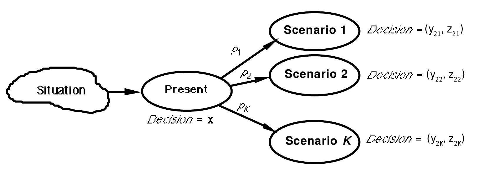
We proceed as usual when modeling a problem, by defining variables. Let x1 ≥ 0 and x2 ≥ 0 be the number of units of products A and B to produce now (at the first stage), respectively. As we have a set of K scenarios we associate a scenario subscript with the recourse variables at the second-stage, so let y2k ≥ 0 and z2k ≥ 0 be the number of units of product A and B, respectively, to buy from the external supplier at the second stage under scenario k, i.e., when the stochastic realization of the demand is Dik (i=1,2; k=1,…,K). We can consider a particular example with two scenarios for the demand, where the first represents a low demand situation for both products (D11 = 400, D21 = 500) with probability of p1 = 0.7, and where the costs of both products from the external supplier are of (c11= 2.5, c21= 2.3), respectively. The second is a top-demand scenario, with demands of (D12 = 600, D22 = 700), costs of (c12 = 3, c22= 2.7), and probability of p2 = 0.3. Note also, that we have looked forward just one period into the future in trying to plan production.
The constraint that ensures the limited capacity of the system is x1 + x2 ≤ 600. And, the constraints to ensure that demand is always satisfied are: x1 + y2k ≥ D1k; and x2+ z2k ≥ D2kfor k=1,…,K.
We must have ≥ here, since the amounts x1and x2we produce may (depending upon the particular demand that occurs) exceed customer demand. For the objective function we have a cost 2x1+ 1.5x2incurred with certainty and K costs c1ky2k+c2k z2k, each incurred with probability pk. Note here that, in practice, only one of these K costs will be incurred, once a realization of the demand occurs.
It would seem natural to minimize the expected cost over the set of scenarios, so that the stochastic optimization model becomes:
minimize 2x1+1.5x2+ ∑ pk (c1k y2k+c2k z2k)
subject to
x1 + x2 ≤ 600
x1 + y2k ≥ D1k k=1,…,K
x2 + z2k ≥ D2k k=1,…,K
x1 ≥ 0
x2 ≥ 0
y2k ≥ 0 k=1,…,K
z2k ≥ 0 k=1,…,K
Note that this is a deterministic problem. This problem is called Deterministic Equivalent Model, DEM, a term coined by R. J-B. Wets in 1974. Note also that we could require x1, x2, y2k, and z2k to be integer. In this case the corresponding DEM is an integer optimization problem or a mixed integer problem if some of them are continuous.
The simplest form of the two-stage stochastic integer DEM has first-stage pure 0-1 variables and second- stage continuous variables. In the general formulation of a multi-stage stochastic integer optimization, decisions on each stage have to be made stage-wise. At each stage, there are variables (decisions) which correspond to scenarios with a common history. Then, these decisions must take the same value under each of these scenarios, i.e., the non-anticipativity constraints, NAC, (also introduced by Wets in 1974) must be satisfied, implying we cannot anticipate the future.
If we want to find the optimal solution we have to solve the above problem. This requires a computer and a solver. In this case, the optimal solution is: x1=100, x2=500, y21=300, y22=500, z21=0, z22=200, with an expected cost of 2087€. This solution means producing now 100 units of product A and 500 units of product B. In the next period, and depending on the demand scenario, buying 300 units of product A if demand is low and 500 units of product A and 200 of product B if there is a high demand.
Solvers are commercial versions of algorithms, i.e., programs to be used on a computer. There are two algorithms that have proved to be key in the solution procedure of most of the optimization problems: the simplex method for solving linear problems and the branch and bound that in combination with the simplex method, has been shown to be an efficient tool to solve deterministic integer problems, at least for moderate dimensions. However, a vast majority of real mathematical optimization problems, whether deterministic or stochastic, require integer variables (and perhaps also binary variables to model primarily qualitative terms), usually in multistage environments with a high number of scenarios, raising the resolution effort by several orders of magnitude. Stochastic problems of this type have dimensions in real-world applications so is not easy for the corresponding DEM can be solved by the direct use of optimizers. Instead it requires the use of decomposition algorithms and parallel computing.
The DEM provides a solution that is feasible for any scenario considered, and, at least, optimizes the expected value of the objective function (which today is called risk neutral strategy). Alternatively, certain risk control strategies (called risk aversion strategies) have appeared in the literature since the late 90s which provide solutions that consider the variability of the objective function over the set of scenarios. These include scenario immunization, value-at-risk, conditional value-at-risk, expected shortfall over thresholds or first-and second-order Stochastic Dominance Constraints (SDC) for a set of profiles, see Gollmer et al. (2008) and (2011).
Finally, note that problems of stochastic optimization are found in diverse areas of mathematical, natural and social sciences as well as in engineering. Many of them originated in real-world applications. Developments in the vast field of optimization are motivated by these applications and have been drawn from both mathematics and computing science over the years. Areas where these techniques are used include capacity planning, modeling strategic capacity investments or power systems, modeling the operation of electrical power supply systems in order to meet consumer demand for electricity, among many others. Probably the current predominant use of multi-stage stochastic optimization models is in the field of quantitative finance. For example the modeling of an investment portfolio in order to meet random liabilities. Stochastic optimization techniques can effectively identify the solution to complex portfolio planning problems with many constraints. Using stochastic optimization we can find feasible solutions to the problem, or demonstrate that a risk exposure target is unattainable.
References
[1] E.M.L. Beale. On minimizing a convex function subject to linear inequalities. Journal of the Royal Statistical Society, Ser. B, 17: 173-184, 1955.
[2] J.R. Birge and F. Louveaux. Introduction to Stochastic Programming. Springer, 2nd edition, 2011.
[3] A. Charnes and W.W. Cooper. Chance-constrained programming. Management Science, 5:73-79, 1959.
[4] G.B. Dantzig. Linear programming under uncertainty. Management Science, 1:197-206, 1955.
[5] R. Gollmer, F. Neise and R. Schultz. Stochastic programs with first-order stochastic dominance constraints induced by mixed-integer linear recourse. SIAM Journal on Optimization, 19:552:571, 2008.
[6] R. Gollmer, U. Gotzes and R. Schultz. A note on second-order stochastic dominance constraints induced by mixed-integer linear recourse. Mathematical Programming, Ser. B, 126:179-190, 2011.
[7] R.J-B. Wets. Stochastic programs with fixed recourse: The equivalent deterministic program. SIAM Review, 16:309-339, 1974.
About the authors
Araceli Garín obtained her PhD. degree at the University of the Basque Country, in the field of Mathematics in 1992. Her main interests lie at Mathematical Programming with and without uncertainty in the parameters. At present she is an Associate Professor at the School of Economics and Management, UPV/EHU at Bilbao (Spain).
Gloria Pérez obtained her PhD. degree at the University of the Basque Country, in the field of Mathematics in 1986. Her interests also lie at Mathematical Programming. Now, she is an Associate Professor of Statistics and Operations Research, UPV/EHU at Leioa (Spain).
Both belong to EOPT, a group doing research in Statistics and Optimization and to GOE, a group doing Parallel Stochastic Optimization. In cooperation with similar groups in Spain, Italy and Norway, they are involved in algorithmic development and applications of stochastic optimization in the finance, power generation and oil industries.