The math of sex and hunger. A short history of population dynamics
The math of sex and hunger. A short history of population dynamics
The field of population dynamics lies between mathematics and biology. Its subject of study is the evolution of biological populations with time. The natural language for dynamical problems is that of differential equations, and population dynamics is not an exception to this rule.
Such a powerful tool was well known since the times of Isaac Newton, so it is not surprising that the field of population dynamics has a history of more than 200 years.
Early developments
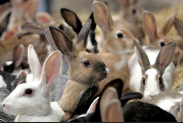
The first reference of a problem on population dynamics is due to Leonardo de Pisa, also known as Fibonacci, who studied the growth and reproduction of rabbits in the early years of the XIII century. He proposed a time-discrete model like this:
- Step 0: we start with a young immature couple of rabbits
- Step 1: the couple of rabbits is now mature.
- Step 2: the couple of rabbits give birth to a second immature couple of rabbits.
The model of Fibonacci iterates again and again without accounting for deaths of the older rabbits. See figure below:
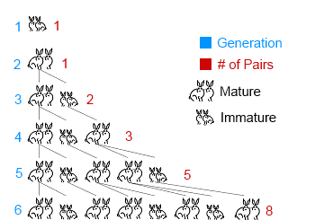
The number of alive couples at each step corresponds to the well known Fibonacci series, which is formed by summing the previous two elements in the list.
- Step 0: 1
- Step 1: 1
- Step 2: 1 + 1 = 2
- Step 3: 1 + 2 = 3
- Step 4: 2 + 3 = 5
- Step 5: 3 + 5 = 8
- And so forth…
Malthusian growth
The book An Essay on the Principle of Population (1798) by Thomas Robert Malthus is considered to be the first scientific approach to population dynamics. Despite it is a book about economics and not about mathematics, it contains the first model of population growth described on mathematical terms.
The underlying idea is very simple: the rate of growth is proportional to the number of living specimens of a species. That is:

being r the proportionality constant, and N the number of specimens. The family of solutions for this equation is a well known one, that of exponential functions.
The meaningful solutions verify that both the proportionality constant and the number of specimens are positive numbers.
The model obviously is only valid for a single species and lacks any interaction between different species. There’s also an important flaw for this model: there is no death. Still, the r term can be calculated as a birth rate minus a death rate, but the model remains essentially the same. This leads to unlimited growth and no equilibrium solutions, which obviously doesn’t occur in nature.
Logistic growth
The next step in the development of population dynamics was proposed by Pierre François Verhulst in 1844. It was the addition of a death term, with a minus sign, to the Malthusian growth equation. This improved model is known as logistic model:

where K is known as carrying capacity for reasons that will become obvious below.
The family of solutions looks like:
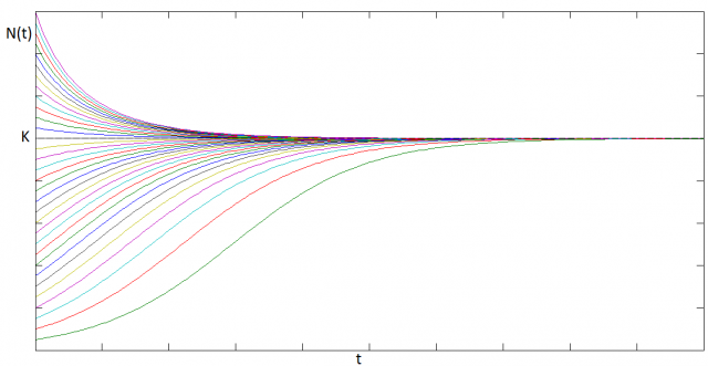
In this case, we have a non-trivial equilibrium solution, i.e:  , corresponding to the maximum population the system can support. This equilibrium is reached always, regardless of the initial conditions.
The logistic growth model is appropriate for modeling, for example, the growth of bacteria inside a Petri dish under controlled conditions, where the resources are clearly limited and there are no seasonal variations of, say, temperature or humidity. Its main flaw is that the model is completely blind to an interaction between different species.
Logistic growth with seasonal variations
A straightforward way for obtaining a more realistic model is adding a periodical dependence of the carrying capacity with time. This is a very simple example of yearly variations due to the different seasons:

The explicit presence of time in the differential equation turns it into a non-autonomous one. This makes it harder to solve analytically. Here we plot a family of solutions obtained numerically:
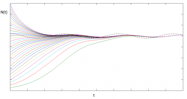
We observe that there’s a stable solution oscillating around the mean carrying capacity, with a phase offset.
This is just a model, but it gives us the flavor of the type of variations we can introduce in order to get better models.
The Predator – Prey model
The first model with interaction between species is due to Alfred J. Lotka and Vito Volterra. Lotka proposed it while studying autocatalytic chemical reactions. Volterra discovered them independently while studying the evolution of the fisheries of the Adriatic Sea.
It had been observed that the populations of the fisheries oscillated with non-yearly frequencies, and it was thought to be caused by the fishing activity. Surprisingly, when World War I stopped almost all fishing activity in the Adriatic, the oscillations prevailed.
So, let’s introduce the mathematical model. Let’s think of a population of foxes F and rabbits R. The idea is that the population of predators is a death factor for the preys, and the population of preys tends to rise the rate of birth of the predators. The predator – prey equations look like:

where all coefficients are positive. α represents the birth rate of the rabbits, and β the likelihood to be killed in an encounter with a fox. δ stands for the probability of a successful hunt by a fox and γ for the rate of natural death of the foxes.
This is a non-linear system. It can be proven that it has periodical solutions, but cannot be solved analytically. Here we plot a possible numerical solution:
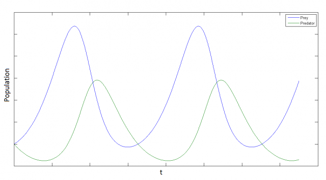
It is interesting to note that the system is intrinsically periodic, even we have not introduced any seasonal term.
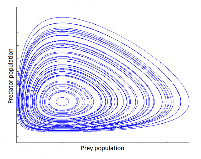
Its phase map is so composed of closed loops:
Further developments
Currently, most of the models are refinements and generalizations of the Volterra-Lotka one. Being even the simpler models non-linear, almost all the models have to be solved numerically. The field is taking advantage of the rising power of computation and the developments of the non-linear systems theory.
The rise of network theory allowed gaining insight into interaction models with more than just two species, treating each species as a node, and each interaction coefficient as a directed edge. This model is known as food web.
Some of the newest models are taking into account the discrete nature of the specimens, using stochastical simulation to model discrete deaths and births, and even mutations (treated as changes in the coefficients, in the simplest cases).
There have been also applications of game theory to this field, usually through more complex simulations taking into account space and not only time.
References:
- George F. Simmons. Differential equations with applications and historical notes. 1991. McGraw-Hill.
- Ali H. Nayfeh, Balakumar Balachandran. Applied nonlinear dynamics. Analytical, computational and experimental methods. 1995. Wiley Series in nonlinear science.
- Vito Volterra. Fluctuations in the Abundance of a Species considered Mathematically. 1926. Nature 118, 558-560
- Stuart L. Pimm. Food webs. 1992. The University of Chicago Press.
2 comments
[…] necesidades diarias, conseguir sexo y no tener hambre. Y, al final, todo se reduce a matemáticas. The math of sex and hunger. A short history of population dynamics, por Pablo Rodríguez […]
[…] La matemática de las relaciones sexuales y el hambre. Una breve historia de la dinámica de la pobl… […]