The value of a statistical life

To avoid any confusion regarding the object of study a disclaimer is in order. A statistical life is not a human life. The value of a human life is a concept that cannot be easily defined, if it can at all. I may value my life in such a way that I am willing to pay all I have and more in order to keep it. Or may be no, since I may be very ill, with very few weeks to live and do not wish to spend all my fortune and leave my children with nothing. Whether others should value my life the way do or in a different way is not the issue of discussion here. Neither is the effort that someone (a group of friends, the State,…) should make to save the life of say a lost mountain climber friend or an astronaut trapped on the Moon after its lunar module has broken.

Most of the decisions regarding the savings of lives are made in statistical terms. At the individual level, one may have to decide whether to accept a highly paid, dangerous job or a safer one with a lower pay. Alternative, there are laws that require people to receive an indemnity after being exposed to an involuntary risk, and a decision must be made about proper compensation. Suppose you are willing to accept the equivalent to 100,000€ for being exposed to a 1% chance of being killed, we then say that for you the value of your statistical live is 10 million euros, the result of multiplying 100,000 times 100.

A related, although different, concept is the value of increasing someone’s life expectation by one year. This is of interest in Medicine: should the public health system invest in another MRI device? Will it save more expected life years than an alternative use of the money? Should the government allocate more money to the health system to save more expected lives? Again, this is not the question we study now.

As stated, one can easily see that the value of a statistical life (VSL) will depend of the size of the perceived risk (one may accept 100,000€ for a 1% chance of dying, but require 300,000€ for a 2% chance), the age of the person making the decision, and many other factors. The question is, then, how to compute a fair average that can guide public policy regarding risks. The remaining of this article explores some of the difficulties of this task and a sample of the strategies followed by researches to solve them. The exposition is not exhaustive, but provides a fair overview of the progress in this topic.

There are two approaches to the question of estimating the VSL. One is the use of revealed preference studies, where researches observe actual decisions and risks. For instance, one may observe salary compensations given to workers that are exposed to fatality risks or price premiums paid for safer automobiles. The other approach is the use of stated preference studies, where individuals are asked to choose between hypothetical risk scenarios.

The empirical data that can be obtained is not always complete, and is subject to bias. For instance, the VST may be underestimated as individuals with a lower risk aversion may accept risks more often and, thus, constitute a disproportionate part of the population from which the revealed preference studies take their samples. The stated preference approach could, in principle, compensate for that.

Viscusi (1993) ¹ and Kochi et al. (2006) ² review a series of works for both types of studies and find the surprising result that, contrary to the observation above, the VSL estimates implied by stated preference studies tend to be lower than those from revealed preference studies and comparison of these studies. This leads to hypothesis that in stated preferences the subjects may be answering a different question (their belief about a societal risk, and not his own, e.g.), and takes researches back to doing more studies.

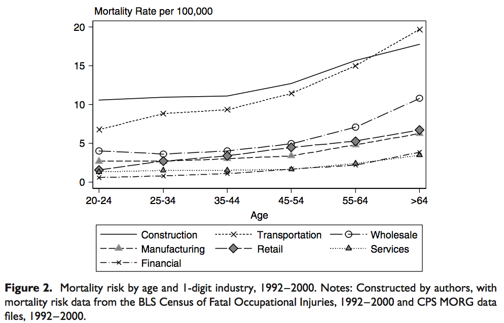
A second problem arises when comparing the observed patterns with the theoretical ones. Based on economic theory, in a world with imperfect capital markets and imperfect insurance markets, the VSL should rise over the life cycle and then eventually decline. This inverted-U-shaped pattern closely follows the trajectory of income and consumption over the life cycle. These empirical data are well explained by the theory that predicts the same behavior for the estimations of VSL along the life cycle. Aldy and Viscusi (2007) ³ reportthat revealed preference studies are consistent with theory, and Krupnick’s (2007) ⁴ shows that stated preference studies are not.

Despite of initial doubts, it seems that revealed preference studies offer better data than the stated preference ones after all. However, we still must not disregard the possibilities of biases.

One of the most salient characteristics of revealed preference studies is the instability of the estimations of the VSL. A notable case in point is the situation of the UK. The meta-analysis by Viscusi and Aldy (2003) identified VSL estimates using UK labor market data of 9.4 million–5.2 million–19.9 million, and 74.1 million, where all estimates are in equivalent dollars of the year 2000. To solve the problem, some authors have tried using better econometric models to treat the data.

Knsiesner et al. (2010) ⁵ use the best econometric technics available to examine the problem. These authors study the differences in the VSL across potential wage levels in panel data using quantile regressions with intercept heterogeneity. Let the words not confuse you: panel data is a set of data collected along time with different observations in each point of time to account different phenomena, the quantile regression is just a regression using the data of the given quantile to account for differences among quantiles, and the intercept heterogeneity is a technique to control for latent heterogeneities, an important problem in econometric studies. Their findings are less unstable and indicate that a reasonable average cost per expected life saved cut-off for health and safety regulations is 8 million per life saved, but the VSL varies considerably across the labor force.

These results also reconcile the previous discrepancies between VSL estimates and the values implied by recent estimations of coefficients of relative risk aversion (Kaplow, 2005) ⁶. Because the VSL varies elastically with income, this work may used to support that regulatory agencies should regularly update the VSL used in benefit assessments, increasing the VSL proportionally with changes in income over time, a point that was overlooked by some agencies.

References

- Viscusi, W.K. 1993. The value of risks to life and health. Journal of Economic Literature 31, 1912–1946. ↩
- Kochi, I., Hubbell, B. and Kramer, R. 2006. An empirical Bayes approach to combining and comparing estimates of the value of statistical life for environmental policy analysis. Environmental and Resource Economics 34, 385–406. ↩
- Aldy, J.E. and Viscusi, W.K. 2007. Age differences in the value of statistical life: revealed preference evidence. Review of Environmental Economics and Policy 1, 241–260. ↩
- Krupnick, A. 2007. Mortality-risk valuation and age: stated preference evidence. Review of Environmental Economics and Policy 1, 261–282. ↩
- Kniesner, T.J., Viscusi, W.K. and Ziliak, J.P. 2010. Policy relevant heterogeneity in the value of statistical life: new evidence from panel data quantile regressions. Journal of Risk and Uncertainty 40, 15–31. ↩
- Kaplow, L. 2005. The value of a statistical life and the coefficient of relative risk aversion. Journal of Risk and Uncertainty 31(1),23-34. ↩