Rapidly Exploring Manifolds: when going from A to B ain’t easy

We will address a recent article by Jaillet and Porta (Institut de Robòtica i Informàtica Industrial, IRI), which reveals new practical applications of highly-abstract mathematical entities.

When it comes to robots, we can’t forget that their fundamental goal is always somehow related to moving stuff. Arm robots as those found in the automotive industries are committed to feeding other machines or to precisely placing tools, e.g. welding guns. Mobile robots, in turn, move their own bodies throughout the workspace.

In general, the position and orientation of a robot with N degrees of freedom can be completely parameterized by means of N coordinates. However, taking the system from some starting configuration q0 to a goal state q1 may be not as simple as it seems. To start with, obstacles may lie in the path so they must be considered to avoid collisions. Secondly, we have nonholonomic constraints. Wheeled vehicles are a perfect example. One easily realizes that the position and orientation of a ground vehicle become perfectly identified by means of three coordinates (a 2D position on the ground plus one angle for the orientation or heading), whereas the vehicle itself (considered as a mechanism) only has two degrees of freedom: the position of each of the two drive wheels. There exists a complex relationship (a differential equation) between the wheel speeds and the position at which the vehicle ends up. Just think about how difficult it becomes to park a car in a narrow slot!

Maneuvering with a car for getting to some desired goal position is one example of the broader family of mathematical problems known as path planning or, more visually, the piano mover’s problem. Put short, the main difficulties arise when we consider that objects can rotate, since the state space in which we must search for solutions becomes of higher dimensionality. Getting out of a 3D maze is harder than doing the same for a 2D maze, right? Now, imagine a six-dimension (or higher) maze… that is exactly the kind of challenge faced by motion planners in robotics.

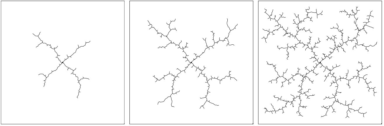
During the 1990s, researchers discovered that integrating randomness in this gigantic search process is a good idea. Rapidly exploring random trees (RRT) ¹ are tree-like structures built by picking random “goals” in the reachable space, then checking if the path to the so-far tree is free of obstacles and in that case adding a new edge, thus expanding (or growing) the tree.

A real application of RRTs is shown in the following video for an automated forklift:

RRTs methods are popular nowadays because they work well in many applications. But now, what would happen if we impose additional constraints to the problem? For example, imagine we need to plan the trajectory for the arm of a robotic waiter which must hold dishes horizontal all the time. Then, picking random configurations for building a random tree is doomed to fail, since only a tiny fraction of all possible configurations fulfill all the constraints. In fact, we have a probability of zero of picking a valid point which, however, doesn’t imply it is absolutely impossible.

Clearly, we need something different when constraints exist. The proposal of Jaillet and Porta, recently published in the journal IEEE Transactions on Robotics ², heavily relies on understanding the abstract geometry of manifolds. It turns out that the state space of all allowed configurations is a manifold, hence the relevance of the concept.

But, what are manifolds? Informally, you can think of them as spaces (2D, 3D and so on) which seem Euclidean locally and which “live” embedded into a larger-dimensionality space. A perfect example is the surface of our Earth: it is a 2D manifold since, well… it’s a surface, right?! But it “lives” in a 3D world, so it has a curvature which, however, is very small and can be only noticed when we take into account very large portions of the surface. If we pick a small area of the surface we could approximate it very well as a perfectly planar surface.

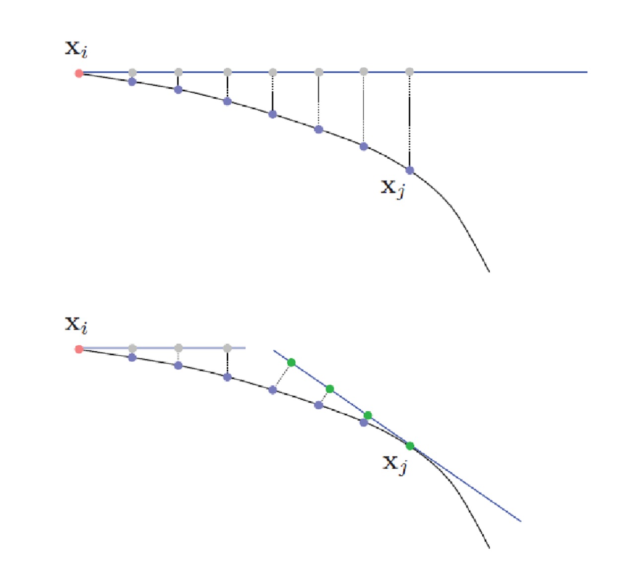
With this idea in mind, we can take an entire manifold and build a so-called atlas of linear approximations (called charts of the tangent space) at some discrete set of locations:

In their paper, Jaillet and Porta propose an algorithm that interleaves RRT with the construction of the atlas of the manifold associated with the kinematic problem at hand. Since the error introduced by the linear approximation (the chart) of the manifold at a given point increases with the distance to its center, they propose a set of heuristic for determining when we should determine the frontiers between the different charts.

The clear advantage of this proposal is that we can now rely on the existing charts to generate new random configurations, which will be valid given the constraints and which allow running the “classic” RRT algorithm for obstacle avoidance.

Among the experiments on which the method has been applied we can find the kinematic problem of finding out how to “blend” a given molecule between two stable configurations:

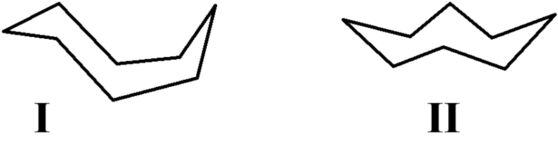
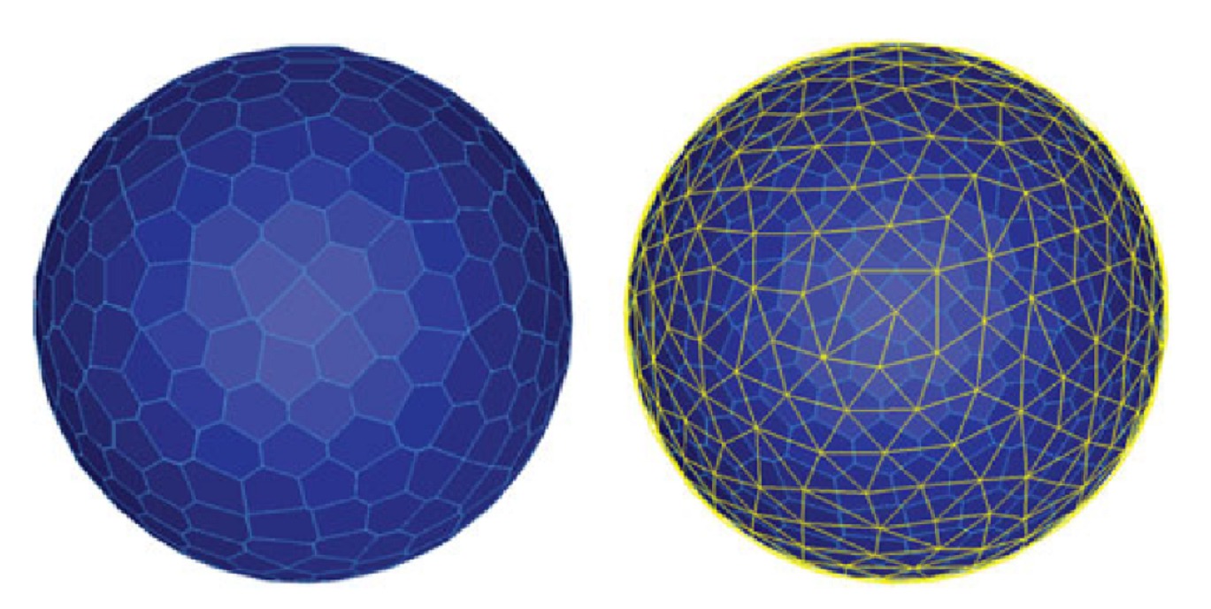
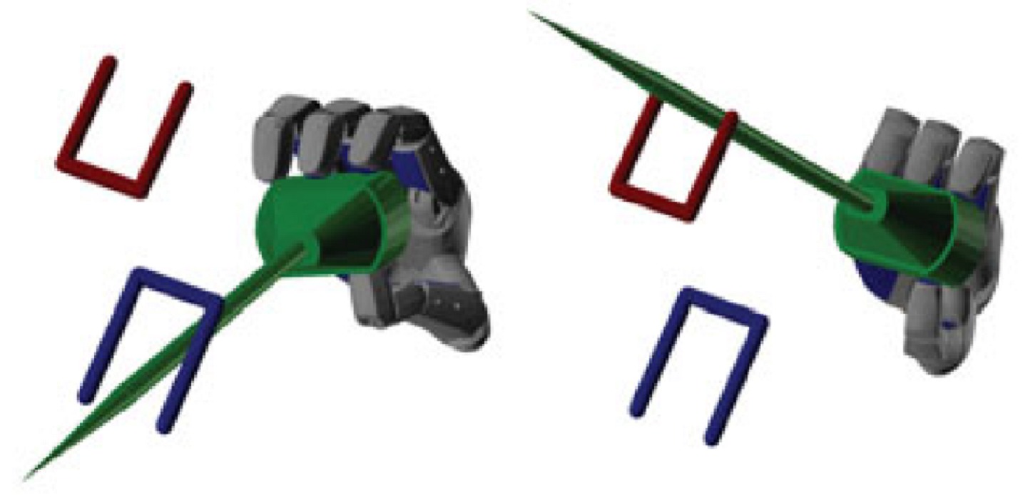
Finding a path between the two configurations of cyclooctane in the table above took 1.94 seconds with the proposed algorithm, in which 139 charts and 5812 nodes in the manifold of the possible configurations of the molecule were evaluated. For comparison, we can see the method applied to planning of one robot hand in the figure below, which took 8.23 seconds despite requiring fewer charts (50) and nodes (1503).

All in all, this new approach seems promising for efficient and robust motion planning of both mobile robots and robotic manipulators. Putting this together to the fact that authors have released an open-source implementation of the method, this will probably become a popular solution in future robotics designs.

References

- S. LaValle, “Rapidly-exploring random trees: A new tool for path planning,” Technical Report 98-11, Iowa State University, Ames,IA, Oct. 1998 ↩
- Jaillet, L.; Porta, J. M.; , “Path Planning Under Kinematic Constraints by Rapidly Exploring Manifolds,” IEEE Transactions on Robotics, vol.29, no.1, pp.105-117, Feb. 2013. doi: 10.1109/TRO.2012.2222272 ↩