Shortcuts for efficiently moving a quadrotor throughout the Special Euclidean Group SE(3) (and 2)

We devoted the first part of this article to introducing the problem of motion planning for autonomous vehicles at a qualitative level and to briefly describing two of the most commonly-used algorithms, RRT ¹ and RRT*² . Next, we will continue getting into deeper mathematical details about the topological structure of the state spaces associated to motion planning.

One of the most time critical steps in RRT, and especially RRT*, is the nearest neighbor search during tree construction, from each randomly-picked pose to the existing tree nodes. In planning for Euclidean workspaces (ℝ² or ℝ³), a universally adopted optimization is the usage of kd-trees, which we will explain next. However, such index trees do not work in curved spaces such as orientations in 2D or 3D. Therefore, we will firstly explain what we mean with “curved spaces”, then will introduce kd-trees and finally will explore some of the proposed modifications to enable their usage in curved spaces.

Mathematically, a three-dimensional point x can be seen as an element of the common 3D Euclidean space ℝ³. We could left-multiply this point x, seen as a 3×1 vector, by a 3×3 matrix M to obtain a modified point x’.

One could use any arbitrary matrix R corresponding to any change of basis, but only some especial matrices represent “rigid rotations”. It can be shown that, in order for a 3D object to be transformed and maintain its scale, angles, and symmetry, a necessary condition is that columns of R must be an orthonormal basis and its determinant must be +1.

In group theory, we call GL(3, ℝ) to the group of all real 3×3 square matrices, from which rotations are only a small subset. Such subset is so important in mechanics and geometry that it deserves a name of its own: the special orthogonal group, or SO(3) for the case of 3D points. Note that, although any such matrix has 3×3=9 elements, we cannot choose all the values arbitrarily, since the rotation of a rigid body in 3D only has 3 degrees of freedom; in other words, there are 9 elements and 6 implicit constraints. Technically, we say that SO(3) is a 3-manifold, a manifold with 3 degrees of freedom, isomorphic to the group of rotations of the Euclidean 3D space and embedded into the 9-dimensional space GL(3, ℝ). For those unfamiliar with manifolds, one easy way to visualize them is the classic example of the 2-manifold corresponding to the Earth surface, embedded into the three-dimensional Euclidean space.

So far we only mentioned rotations, but a body in 3D can be also translated. There exists a compact notation that allows representing both, rotations and translation, in one single 4×4 homogeneous matrix, at the cost of adding one extra row with a constant “1” to any 3D point.

By the way, one of the little things that your computer graphical card knows how to do is multiplying by these 4×4 matrices, an operation that is at the core of any modern 3D game.

We call Special Euclidean group, or SE(3), to the group of all 4×4 matrices that represent valid translations and rotations for ℝ³. Topologically, SE(3) is the semidirect product of groups SO(3) and ℝ³, as a manifold, it is a diffeomorphism of their product SO(3) x ℝ³ . Both SO(3) and SE(3) are also Lie groups, but the implications are not in the scope of this short article.

So far, you should have one idea clear: if we want to make a quadrotor or an autonomous vehicle to describe a predefined path, such path must be computed by finding collision-free paths throughout a space whose topological structure is SE(3), hence the importance of that group, which as we saw can be decomposed into its Euclidean part (translation, in ℝ³) and its curved-space part (orientation, in SO(3)). In the case of articulated or humanoid robots, the problem is even more complex, so we will focus on the simplest case of the vehicle being a single rigid body.

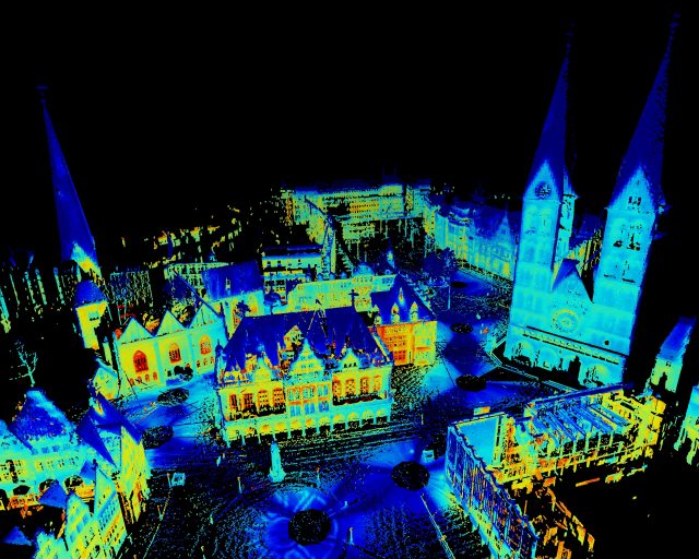
We will now focus on how to find nearest neighbors (NN) for a point in the Euclidean part of the problem. In principle, given any arbitrary set of N points, the only way to tell which is the closest to a query location is checking the distance one by one. This is known brute force search and always succeeds though it obviously has an execution time complexity of O(N). That is, the time required to solve a query doubles if the number of points doubles. Exactly the same NN problem appears in a number of scientific and engineering applications, for example, building large maps of 3D points by gluing together several LIDAR scans to reconstruct a real-world scene.

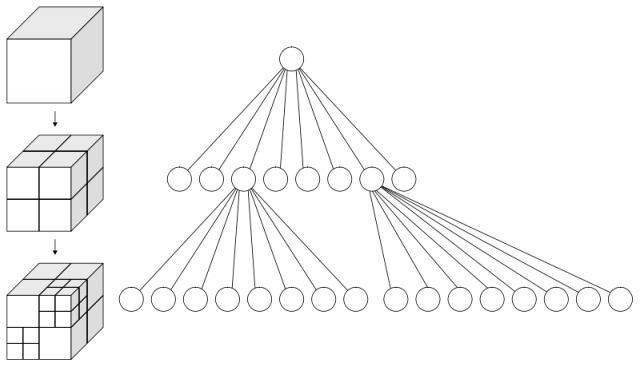
Naturally, there are more efficient ways to solve an NN query. One of the most common optimizations is partitioning space in a hierarchical way in a tree-like data structure. With such a tree, solving a query becomes choosing, at each node (a “volume” of space), the child node in which the query point belongs to, going down the tree recursively. Among these techniques, we have k-d trees (explained later) and octrees (in which each node subdivides its volume into the eight volumes delimited by planes parallel to X, Y and Z).

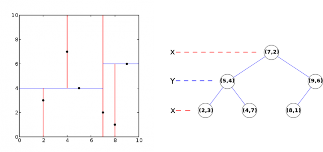
Regarding kd trees, they are a especial kind of binary search tree, widely-used in the problems at hand (and many other field, like pattern recognition in computer vision, etc.) for their ability to balance the space subdivisions according to the real placement of data points. For each node added to the tree, excepting the leaf nodes, the assigned volume is split into two halves along one plane or hyperplane, usually normal to either the X, Y or Z axis. Then, the node is assigned two children nodes, one for each half of the volume, and the process is repeated recursively. One can find two variants of the algorithm, depending on whether the split plane is placed exactly over an existing point, or over some other statistics (e.g. mean). The next figure shows an example of a kd tree construction for a set of 2D points.

Sorting all those points like this is worth the work: afterward, searching for nearest neighbors in a kd tree can be typically achieved in logarithm time, O(log N), an impressive improvement with respect to O(N) of brute force search. For example, it means that instead of doing 1000 or 10000 comparison operations by brute force, we will have to do just 3 or 4 of them along the tree, respectively.

In spite of their advantages, these trees are limited by the assumption that their working state-space is Euclidean, hence they cannot be directly applied to curved spaces like SO(3) or SE(3), where motion planning for vehicles and robots takes place. Here we arrive at the latest proposals in the technical literature to extend kd trees so they work in the problematic part of SE(3), namely SO(3), hence becoming useful in RRT/RRT* planning.

The first proposal came from Yershova & LaValle ³. Their idea to enable kd-trees on SO(3) is fairly simple: to build the tree on the 4-dimensional space of quaternions. Quaternions are an extension to complex numbers, but including three “imaginary” orthogonal axes (i,j and k) instead of the unique “i” of complex numbers. Just like multiplying unit complex numbers can be seen as rotations in the 2D plane, it can be shown (Hamilton) that a rotation of q radians around a direction given by a unit vector (vx,vy,vz) can be represented by a quaternion where the four components form a unit vector in a 4-dimensional space. Topologically, the space of all possible unit quaternions is isomorphic to SO(3) and form a 3-sphere of unit radius in a 4-dimesional Euclidean space, with the peculiarity that antipodal points in the sphere are identified (they touch to each other), just like the 0º and 360º points on the unit circle. That is the reason of the common convention of only using positive values for q_r since negative rotations can be obtained by the antipodal quaternion: with a positive angle along an inverted axis of rotation.

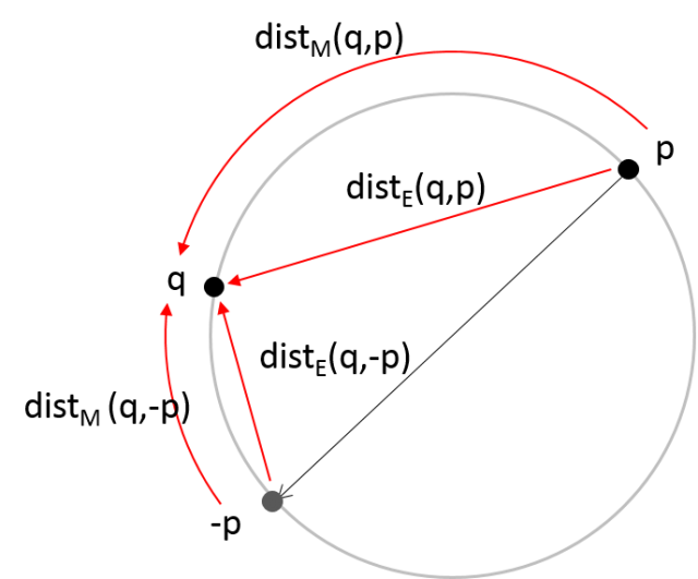
These antipodal “shortcuts” must be taken into account when measuring distances. Yershova & LaValle (2007) proposed to build kd trees just like if points (quaternions) really lived in a Euclidean space, then take into account the non-Euclidean nature just when evaluating distances by the usage of an appropriate metric function. Therefore, the geodesic (over the manifold) distance d_M(p,q) between orientations p and q, is taken as the minimum between the manifold distances from q to p and to –p, which stand for the same orientation. Furthermore, if we only want to find out closest points, not absolute distance values, it is enough to measure Euclidean distances (going “trough” the manifold) instead of “geodesic” ones, as illustrated with the following picture which should be interpreted as a two-dimensional slice of a 3-sphere in ℝ⁴ along the plane that passes through the center in the other two dimensions.

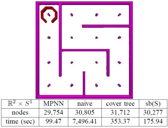
By means of this simple “trick”, the authors showed that a kd tree was more efficient in solving nearest neighbors than other generic search approaches based on user-defined metric distances as “black-boxes”, like cover trees⁴ or “sb(S)”⁵ . Their method, therefore, enabled a computer to solve puzzles like those shown in the next figure in a reasonable amount of time. Yes, that is the real state of motion planning in artificial intelligence (or was, by 2006), do not trust SciFi movies too much…

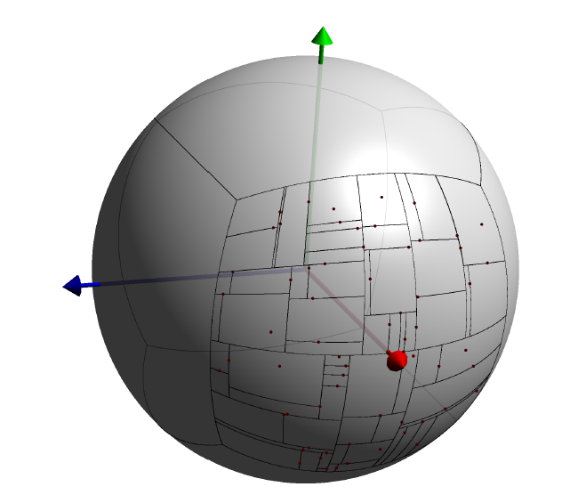
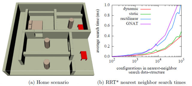
More recently, a new improvement has been proposed by Ichnowski & Alterovitz ⁶. Authors realized that, by partitioning the SO(3) space in 4 “volumes” and building a kd tree for each one, the trees led to more efficient queries for nearest neighbors. The four volumes correspond to the 4 faces of a 4-dimensional cube (tesseract), projected onto the 3-sphere. Since high-dimensionality geometry is hard to picture, one convenient alternative to visualize it would be moving to a 3-dimensional simile: imagine a regular cube (3D), whose faces are projected to a regular sphere (2-sphere). Then, a kd tree is to be built for each “patch” of the sphere corresponding to a cube face. To complete the picture, remember that in the real 3-sphere, antipodal points are identified (due to the properties of quaternion-based rotations), thus that only one of each opposite faces needs to be mapped: 3 for the cube, 4 for the tesseract.

Additionally, authors reported another optimization regarding the hyperplanes that split each node in the tree: classic kd trees always take hyperplanes aligned to the global Euclidean axes. However, by “tilting” them such as they always pass by the origin, the trees are more balanced and queries are more efficient on average.

Hopefully, the reader may now have a better grasp of the kind of mathematical and algorithmic details behind state-of-the-art robots and autonomous vehicles. As a good way to end this entry, let us show to you a spectacular demo on path planning with the CC-RRT* algorithm for a ground robot, performed by MIT Aerospace Controls Lab (ACL):

References

- LaValle, Steven M.; Kuffner Jr., James J. (2001). “Randomized Kinodynamic Planning” (PDF). The International Journal of Robotics Research (IJRR) 20 (5). doi:10.1177/02783640122067453 ↩
- S. Karaman and E. Frazzoli, Sampling-based Algorithms for Optimal Motion Planning, International Journal of Robotics Research, Vol 30, No 7, 2011. http://arxiv.org/abs/1105.1186 ↩
- Yershova, A., & LaValle, S. M. (2007). Improving motion-planningalgorithms by efficient nearest-neighbor searching. IEEE Transactions on Robotics, 23(1), 151-157. ↩
- A. Beygelzimer, S. Kakade, and J. Langford. Cover trees for nearest neighbor. 2004. ↩
- K. L. Clarkson. Nearest neighbor searching in metric spaces: Experimental results for sb(s). 2003. ↩
- Ichnowski, Jeffrey, and Ron Alterovitz. “Fast Nearest Neighbor Search in SE (3) for Sampling-Based Motion Planning.” Algorithmic Foundations of Robotics XI. 2015. 197-214. DOI: 10.1007/978-3-319-16595-0_12 ↩