One way Google’s cars localize themselves

Localization, or knowing “where am I” is a central topic of research in mobile robotics today, and it has been like that for more than 30 years. One cannot conceive ordering a futuristic personal assistant robot “go to the coffee machine and bring me a large one” if the robot is unable to know where it is at each instant during its motion, so it can plan ahead what should be its next steps. Wandering around may be fine for robotic vacuum cleaners, but we cannot go much farther without making machines much more intelligent than that.

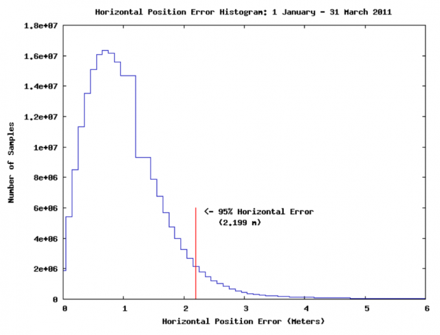
Obviously, future cars able to drive themselves must also know where they are so they can maneuver in time to take a given exit at the highway, respect lanes in one-way streets and so on. This poses two challenges: (1) the car must stay localized againstsome kind of map and (2) localization should be efficient, robust and in real-time.The reader may be tempted to think that current GPS-aided navigation systems (commonly called just “GPS”) are perfectly accurate and a mature technology since, well… we humans use them as a guide every day without problems, right? To fully appreciate why existing GPS systems are not the solution, imagine trying to drive with your eyes blinded, just following the GPS instructions and knowing your GPS coordinates. Without perceiving the environment, the pedestrians, the other cars, temporary works in the road, out-of-date maps in the navigator, etc. I bet it will be not a long way… In addition, GPS accuracy is not as fine as most people assume, being 95% of the time only better than 2 meters, if using the GPS satellite information alone. In narrow two-way roads that is just an unacceptable and dangerous error.

So, GPS is fine as a complement, but we should not rely much on it. We humans are very visual in the way we perceive the world, so allowing future cars to literally see their environment would indeed provide tons of rich information for localization. Most researchers in the field know the famous anecdote about how the Artificial Intelligence pioneer Marvin Minsky mentioned directed an undergraduate student to “solve the computer vision problem” during one summer… in 1966. We are still waiting the end of that long summer! As a side note, Minsky is mentioned in “2001: A space odyssey“, a movie he advised as AI scientist.

Despite the huge progress in computer vision, especially in the last 10 years, we all know in the field how brittle and limited are all current methods in comparison the immense capabilities of the human brain for interpreting and understanding images. In short: it is still not safe yet to rely self-driving cars on cameras and computer vision techniques.

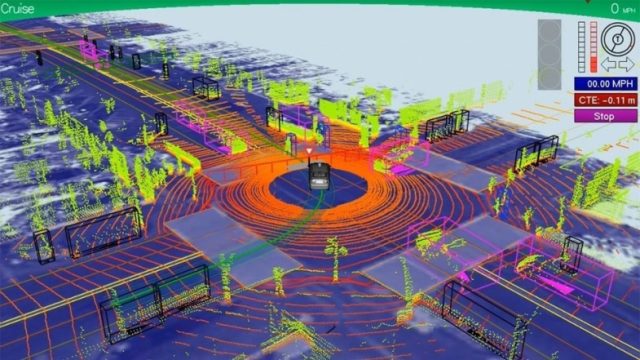
At present, the most valuable sensor for autonomous vehicles are 3D laser scanners, or LIDARS. They provide a 3D scan of the environment, with range (depth) and reflectivity information for each direction in the space. Despite their absolute unsuitability for market cars (each LIDAR costs ~$70,000 or more) they are popular in research labs around the world, including Google’s. The following video from a real experiment illustrates how the world looks like with “LIDAR eyes”:

This is how a state-of-the-art autonomous car “sees” the world

The work¹ introduced one robust technique to localize a vehicle using such LIDAR sensors. It was coauthored by renowned Sebastian Thrun, head of the Google’s self-driving car project, and prolific researcher in mobile robotics (54k citations and 113 h-index!). Although the paper only assured that the technique was in operation during 10 autonomous driving tests in the Stanford campus, we can infer that it may be part of current software in Google’s cars.

Following the tradition in mobile robotics, localization is feasible only after building a map of the environment, which is then used as a reference for localization assuming the environment will not change too much. There are strong reasons to work like that: building a map is one of the most difficult problems in robotics and computer vision (a problem known as SLAM), so we researchers normally collect data by driving the vehicles manually, then spend a while in the office tweaking parameters of map building methods until we are satisfied with the accuracy of the resulting map, and only then, feed the map to the localization methods which will run in real-time on the vehicle.

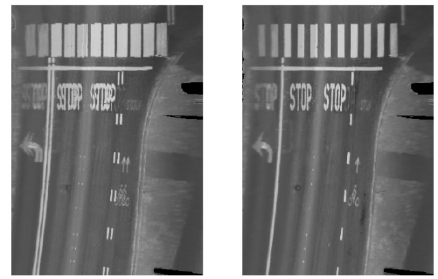
In the case of this work by Thrun’s team, the dense 3D point cloud from the LIDAR is enhanced with its “color” as seen by the laser: by monitoring the intensity of echoed infrared laser beams, the sensor knows the gray level of each point in the surroundings, determined by its reflectance. Composing 3D points with this information leads to gray scale photorealistic images of the world, as that shown in the next figure. It is worth insisting in the fact that gray levels were not captured by a camera, but scanned one point at a time (millions per second) by the LIDAR.

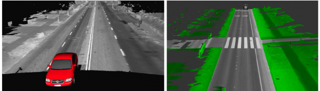
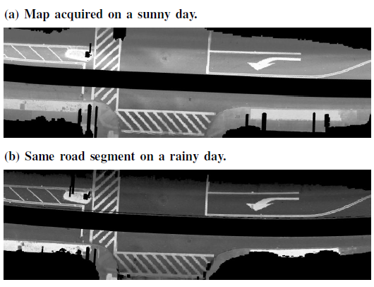
Then, just the ground plane part of this map is kept for localization. According to the authors, taking into account the full 3D structure of the world did not help much. Since these ground “images” are not grabbed with normal cameras, some typical pitfalls and problems of imaging are avoided. For example, there are no sunlight shadows; remember we are directly measuring reflectance of points with a LIDAR. Also, the obtained images only change slightly with weather conditions.

Taking two or three rides with the car while grabbing data is just the first step, and the easiest one, of building the map. Now, we have a bunch of Gigabytes of data including millions of 3D points, noisy GPS coordinates and proprioceptive data like inertial readings, the equivalent to human’s internal ear, and wheel encoder readings or odometry (the count of how many times the wheel turned over time).

Since Carl F. Gauss we know that least squares minimization is an excellent tool to fit any model to an experimental dataset, and a map of a city is simply a case of a mathematical model. This least-squares approach is known in the community as Graph SLAM . The “graph” in the name follows from the interpretation of the problem as a network where nodes are car positions and map portions, while edges between nodes are constraints that model the different readings that relate neighboring positions (e.g. by counting wheels turns or by matching two map patches). All in all, the problem reduces to minimizing this cost function:

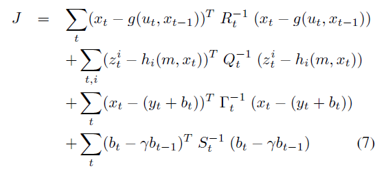
where x are car positions, g() is the odometry model, h() is the observation model that predicts the appearance of the ground as seen from each x, m is the map of the ground itself, z the LIDAR readings, y are GPS readings and b is an ingeniously-proposed latent variable that models the slowly changing bias in GPS signals. The idea is to adjust all car poses x and map values m such that they fit the observations of all sensors simultaneously. Since not all sensors are equally reliable, weighting matrices (all appear as inverted matrices above) are used to ponder the contributions of each term.

A really nice model. The problem is, it is intractable. With millions of unknowns and observations, it may take forever to optimize it. So, the Stanford group proposes to filter out the map from the estimation. Similar to a classic divide and conquer strategy.

Firstly, a simplified model is addressed: by just using GPS and inertial data, we have a first estimation of the car path. Assuming that the orientations are then approximately correct, only small errors in translation remain, which are much easier to estimate since they do not introduce nonlinearities as orientation changes do. Then, the maps of the ground plane built every time that the car passes over the same place (a loop closure in SLAM parlance) are matched to each other to establish additional constraints between vehicle positions. By doing so, we discard the observation function h() above and can focus on optimize just the trajectory of the vehicle. A much simpler cost function:

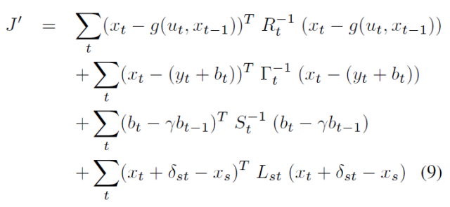
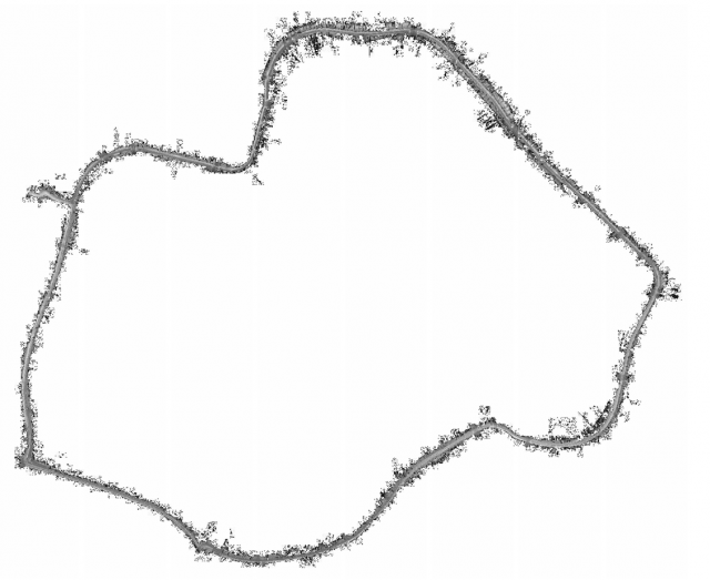
This problem has orders of magnitude fewer variables than the original one, and can be solved in a few seconds. The result is a near perfect alignment (typical errors around 5cm) between different passes of the car over the same places:

Once we have the correct trajectory of the car, building the complete ground map becomes the trivial geometric problem of projecting the laser measurements from known positions and orientations.

Finally, we can drive the car and it will be able to localize itself with a high accuracy thanks to this map. To do so, a particle filter (PF) is employed, which compares LIDAR readings with the ground map. A PF is a particular instance of Bayesian estimator, very similar in its workings to genetic algorithms… but with a solid mathematical and statistical foundation: the vehicle position is estimated by a set of hundreds of hypotheses which evolve over time following the different possibilities that are compatible with the noisy measurements of odometry, inertial readings, etc. Each hypothesis will predict different LIDAR readings, and those that more accurately match the actual data survive; the rest are discarded.

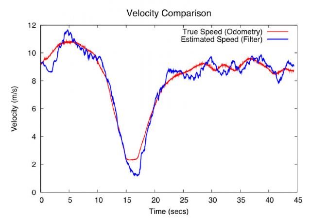
In spite of the simplicity and limitations of this kind of filters, they have demonstrated to be extremely robust against noise and unexpected events in the task of localizing a mobile robot or a car against a known map. In [1], the Stanford team even demonstrated that a PF without odometry nor GPS, only with LIDAR and inertial data, is perfectly capable of tracking the vehicle position, and its velocity, over time.

To sum up, we are still far from seen autonomous cars in our cities because of the extremely expensive LIDAR sensors required by state-of-the-art prototypes… but 15 years ago even Google car seemed sci-fi, so stay tuned 😉

References

- Levinson, Jesse; Montemerlo, Michael; Thrun, Sebastian. Map-Based Precision Vehicle Localization in Urban Environments. En Robotics: Science and Systems III. 2007. ↩