Shortcuts for efficiently moving a quadrotor through the Special Euclidean Group SE(3) (1)
Shortcuts for efficiently moving a quadrotor through the Special Euclidean Group SE(3) (1)
Undoubtedly, the most popular aspect of driverless cars, autonomous drones and quadrotors are the cool videos we are getting accustomed to seeing around. However, behind each of those spectacular demonstrations there is a large amount of work, both practical and theoretical. In this series of articles we will shed some light on one of the most unknown topics by the general public: the mathematical intricacies related to the fact that we live in a three-dimensional world, how that complicates the planning 3D paths and some recent related advances.
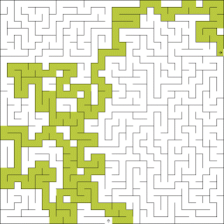
We are all familiarized with the two and three-dimensional Euclidean space, mathematically denoted as ℝ2 and ℝ3, respectively. To specify the location of a point in those spaces, we know it is enough to give its two or three coordinates, e.g. Cartesian coordinates. An example of path planning for points in such space that is familiar to most of us is the classic two-dimensional maze puzzle we can find in magazines. If we take a pencil and mark the way out of the maze, we would obtain a trajectory consisting in the sequence of locations a point must traverse in order to solve the puzzle.
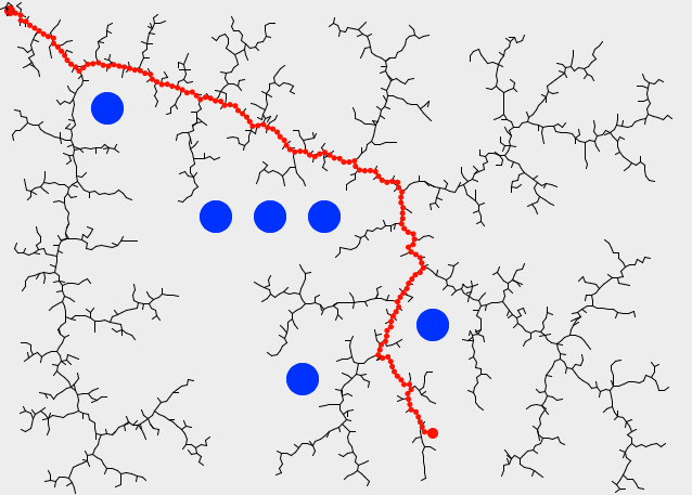
In the fields of Artificial Intelligence and Robotics, we have had efficient algorithms capable of finding obstacle-free paths that take a point-like object from “A” to “B”. For example, Rapidly-exploring random tree (RRT) 1 was introduced in 2001 and has quickly become a seminar work. The method proposes the constructions of a tree of trajectories, which grows by randomly picking collision-free locations in the space, then selecting the closest point in the tree (we will see much more on this “closest” in the next part of this article) and creating a new edge along such shortest path.
Complications start to appear when we move from dealing with “mathematical points”, elegant abstractions that have little in common with the real solid bodies of flying machines or autonomous robots with a finite three-dimensional extension. Then we realize that in order to know exactly the position of a solid, three Cartesian coordinates are not enough to know whether the body collides with some obstacle: we must also specify its orientation. Orientation and angles, those are the sources of all the difficulties. If we also bring into the picture kinematic constraints (e.g. the fact that a common car can only move in a direction determined by its front wheels) and dynamic constraints (e.g. a quadrotor flying at 1 m/s cannot always make a U-turn as steep as one may want), motion planning becomes much more interesting. A lot of research work is being done at present around those areas, and we might visit them in future posts.
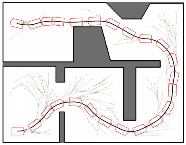
In the present post, we will only focus on complications that arise due to the existence of orientation in vehicle path planning. As an example of maneuverings found by an autonomous planning method, taking into account the real shape of a vehicle, the next figure shows the path found by a variant of RRT presented in 2, for realistic kinematic constraints, namely, Ackermann drive kinematics.
Regarding the RRT algorithm, the reader might have noticed that in its definition we said that target points were selected “at random”. This turns the algorithm into a nondeterministic one: each time one runs the method, a totally different path is obtained and, although all lead to the goal, it is almost sure that the optimal path will never be found.
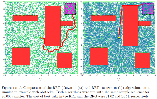
Therefore, in recent years RRT is being replaced by the usage of its variation RRT* (read “RRT star”). Introduced in 2011 in 3, this improved RRT also picks points at random, but then uses them to improve all the path segments around that point and the closest tree edges. Interested readers can check out this simulator comparing RRT and RRT*. The longer one runs RRT*, the better the obtained path will be. This is a property of the so-called anytime algorithms.
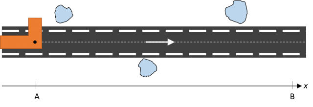
To help illustrating the differences between planning with real vehicles and the classic maze puzzle, at a mathematical (topological, actually) level, let’s imagine the following situation: we must drive a vehicle carrying an “L”-shaped piece onto it though a very narrow road. You can picture it as a Tetris’ part on wheels. The goal is taking the part from “A” to “B” avoiding collisions with nearby obstacles, with allowed movements being: moving forward (to the right), rotate clockwise and counterclockwise.
One of the possible solutions is the next sequence of movements:
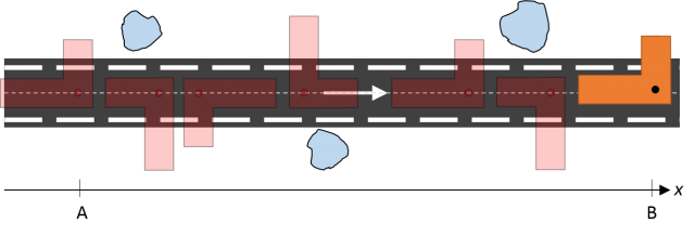
We can model the trajectory of the part along the horizontal axis as one single coordinate “x”, which belongs to the one-dimensional Euclidean space ℝ1. What happens with the angle, or orientation of the part? One could parameterize its orientation by means of its angle “α” to the horizontal line, which then would range from -180º to +180º to span all possible orientations. Setting the original orientation of the part at “A” as reference (angle α=0º), and following its rotations toward “B”, it can be seen that it completes an entire counterclockwise rotation of 360º. So, we shall have α=360º, in spite of it being exactly the same than the starting orientation α=0º.
This means that, even for such simple scenarios, we must account for the topology of the state space. It is not enough to say that the part is moving along coordinates q=(x, α), we must specify that , that is, its topology is the product of the one-dimensional line and the topology of the unit circle, in which the two ends (0º and 360º) are exactly the same point.
Perhaps the reader is surprised by the unnecessary cumbersome notation for such a simple problem: “Why cannot programmers just take the 360º (or 2±π radians) modulus for all angles?” “Is this such a big deal?” Actually, it is. The topology of the state space must be taken into account in many situations, one being the search for the nearest neighbors in the RRT/RRT* tree from randomly-picked poses. During such a search, one should consider not only the Euclidean distance in the space but also the “rotation distance” between two orientations, and even for planar rotations one must correctly handle the discontinuity at 0º (or ±π radians, whatsoever) to detect that 5º is only 10º apart from 355º.
Nevertheless, it is only when we move to the real 3D world when things got more serious and there is no alternative to fully understand the mathematical details of space transformations, what are the Special Orthogonal groups SO(N) and Special Euclidean groups SE(N), and how modern path planning algorithms handle their topological peculiarities. We will discuss all those topics in the next part of this series.
References
- LaValle, Steven M.; Kuffner Jr., James J. (2001). “Randomized Kinodynamic Planning” (PDF). The International Journal of Robotics Research (IJRR) 20 (5). DOI: 10.1177/02783640122067453 ↩
- J.L. Blanco, M. Bellone, A. Gimenez-Fernandez, “TP-Space RRT: Kinematic path planning of non-holonomic any-shape vehicles”, International Journal of Advanced Robotic Systems, vol. 12, no. 55, 2015. DOI: 10.5772/60463 ↩
- S. Karaman and E. Frazzoli (2015) Sampling-based Algorithms for Optimal Motion Planning, International Journal of Robotics Research, Vol 30, No 7, 2011. DOI: 10.1177/0278364911406761 ↩