The geometry of String Theory compactifications (I): the basics.
The geometry of String Theory compactifications (I): the basics.
This is first of a series of notes on the geometry of String Theory compactifications. The space-time in String Theory 12 is often described by means of a mathematical object called manifold 3. Manifolds are very important objects from the mathematical and the physics point of view, not only in String Theory. For example, differential geometry, an important branch of mathematics, studies manifolds as interesting objects by themselves, usually equipping them with some extra-structure, like a symplectic form, a complex structure etcetera. On the other hand, manifolds are successfully used in experimentally proven physical theories4, like General Relativity or Yang-Mills theories. Let us start by giving a somewhat informal definition of manifold:
A manifold M is a set of points equipped with some extra-structure, called the atlas of M, which guarantees that locally it is equal to flat space of some given dimension n. It is said then that the manifold is n-dimensional.
Intuitively speaking, a manifold M is an object that locally, that is, if one gets close enough to it and focus on a small enough portion of it, looks like flat space of a given dimension. The dimension of the flat spaced used to locally model the manifold is then said to be the dimension of the manifold. Here by flat space of a given dimension we mean a higher-dimensional generalization of the standard real plane, which would be then two-dimensional flat space. The atlas identifies a small neighbourhood of every point p in M with a given piece of flat space, assigning to every point p in M a unique point i in the corresponding flat space, whose coordinates are then said to be the coordinates of p. Flat space is by itself an example of a manifold, of course. Let us take the plane P as an example again. Since it is already flat space, the atlas can be taken to be the identity, namely, each point is identified with itself by it.
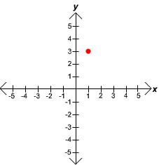
Given two perpendicular axis x and y, we need two numbers, say a and b, to specify a point p in P. The red dot in figure 1 for example corresponds to the point (1,3). These are the coordinates of the point respect to the axis, which is then said to be a system of coordinates for P. Since this system of coordinates covers the whole P, to do so we only need to extend each axis to infinity, it is said to be a global system of coordinates, and since P does not stretch or bends it is said to be flat. This can be seen simply by noticing that the global system of coordinates x and y are straight, lines.
Another simple example is the Euclidean space E, or the spatial space of everyday experience:
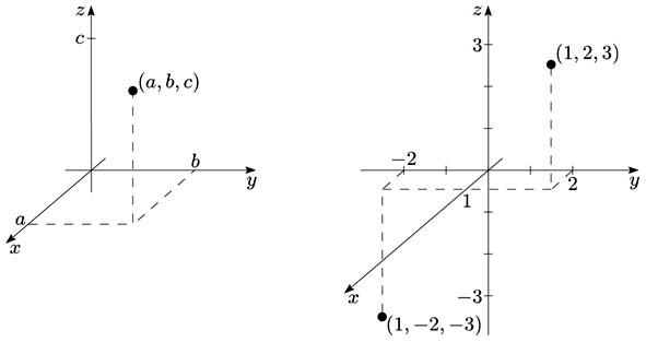
As in the two-dimensional flat case, there is a global system of coordinates, given this time by three axis, the axis x, y and z. Using this system of coordinates, points in this space are labelled by three numbers (a,b,c) which correspond to their coordinates respect to the axis x, y and z. Therefore, Euclidean space is three-dimensional. Euclidean space is already flat space not only locally but globally: the three straight axis can be extended to infinity covering the whole space without bending.
Let us give now a non-trivial and in fact important example, namely, the sphere. This a two-dimensional curved manifold, as it can be readily seen from its graphic description inside the three-dimensional Euclidean space.
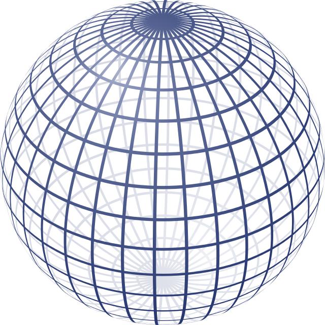
If we get close enough to the sphere, it looks like the flat plane P, as we can see taking the surface of the earth as an approximate example: we are so close to it that for us it really looks like two-dimensional flat space. In fact, it took some time for the human being to realize that the earth was actually not flat. In other words, we can only see a very small portion of the earth and that is why it looks like a flat two-dimensional plane; the same would happen had we lived on any other two-dimensional manifold.
We can also see why the sphere is a two-dimensional manifold from Figure 3. The grid that covers the sphere shows that one can specify a point on the sphere by giving just two numbers, its latitude and the longitude. The grid is a then a coordinate system on the sphere, which bends since the sphere is curved. Notice that in this case, in contrast to what happens in the Euclidean plan or the Euclidean space, the system of coordinates does not cover the whole manifold, which in fact needs an atlas of at least two charts to be correctly described.
The sphere can be easily described in an algebraic way. More precisely, the sphere of radius R can be formally defined as the set of points in three-dimensional Euclidean space that is at distance R from the centre of coordinates, the point (0,0,0). In euclidean space, the distance d(a,b,c) of a point (a,b,c) to the origin of coordinates can be found by a simple application of the Pythagoras theorem and it is given by d(a,b,c) = a2+b2+c2. Since the geometric condition defining the sphere is that it consists of all the points in E at distance R from the origin, the sphere can be succinctly defined as the set of points (a,b,c) in E satisfying:
a2 +b2+c2 = R2
This is the algebraic expression for the standard sphere. Having the algebraic expression of a manifold is extremely useful, since it allows to obtain a lot of information about it, which otherwise would not be easily accessible.
The sphere is also a simple example of a compact manifold, which is a particular class of manifolds of utmost importance in String Theory compactifications, as we will see in a moment. The compactness condition can be intuitively understood using Euclidean space. A manifold embedded in Euclidean space, as the sphere in figure 3, is compact if and only if it is bounded, namely it is contained in a finite size region of E and it is closed, namely it contains all its limiting points.
At this point we have seen three examples of manifolds, one of them non-trivial, the two-sphere. This is an important example of manifold. However, the manifolds appearing in String/M-Theory are more complicated, and in general higher dimensional.
The space-time in String Theory is usually described by a ten-dimensional or eleven-dimensional manifold, depending if we are dealing with Superstring Theory or M-Theory [2], respectively. In any case, in String Theory we need more than the four dimensions of every day experience, namely time and the three standard spatial dimensions. The dimensions beyond the fourth are then said to be the extra-dimensions. In order to fix this mismatch in dimensions, it is usually assumed that the extra-dimensions are so small that we cannot detect them in current experiments and thus that is the reason we have not seen them yet. In particular, it is assumed that the extra dimensions are described by a compact manifold, and that is why the concept of compact manifold is so important in String Theory. Compact manifolds are particularly well suited to describe the extra dimensions because intuitively speaking they are manifolds that are contained in a finite size region of Euclidean space and therefore have finite volume, which we can make as small as we want. More precisely, the ten-dimensional manifold M that models the space-time in Superstring Theory is assumed to be of the form [1,2]:
M = M4 x M6 ,
where M4denotes the standard four-dimensional space of every-day experience and M6 denotes the six-dimensional manifold describing the extra-dimensions. This means that every point p in M can be written as point in M4 , given in terms of four numbers, and a point in M6, given in terms of six numbers, the six extra dimensions. A specific procedure that implements this idea is the Kaluza-Klein compactification, dating almost a hundred years back, see references [1,2,4] for more details and citations to the original references. In the simple Kaluza-Klein scenario, M4 is assumed to be flat four-dimensional space and once this assumption has been made, the relevant problem is to find what are the possible compact manifolds M6 allowed by String Theory. These are the String Theory compactification backgrounds. In order to describe them it is necessary to introduce further structure on our manifold M, aside from its atlas. In particular we will need to introduce the notion of connection, which allows to properly define the concept of curvature, and the notion of metric, which allows to measure distances, among other things. This will be the goal of the next note, where we will explain, among other things, how Calabi-Yau manifolds appears in String Theory compactifications.
References
- Michael B. Green, John H. Schwarz, Edward Witten, “Superstring Theory”, Cambridge University Press, Jul 29, 1988. ↩
- Katrin Becker,Melanie Becker and John H. Schwarz, “String Theory and M-Theory: a Modern Introduction”. January 2007. Cambridge University, Cambridge University Press, 2007. ↩
- Shoshichi Kobayashi and Katsumi Nomizu, “Foundations of Differential Geometry”, 1996, Wiley-Interscience. ↩
- Ortín, Tomás, “Gravity and Strings”. Mar 2004. 704 pp. Cambridge University, Cambridge University Press, 2004. ↩
2 comments
[…] The geometry of String Theory compactifications (I): the basics. […]
[…] The geometry of String Theory compactifications (I): the basics. (mappingignorance.org) […]