Helping Spider-Man to plan his moves efficiently
We all know how Spider-Man moves through the city, shooting spider-webs from wall to wall. But, have you ever wondered if he is actually using the shortest route? And, if so, how does he compute it? Since walls introduce a third dimension into the problem, the algorithms in a usual GPS navigator are no longer useful. Hopefully, the results in a recent paper by Carmi et al. 1 would help to develop a navigator being useful for Spider-Man.

The authors translate the problem into computing a fundamental geometric structure, the so-called visibility graph. This is broadly used in motion planning, see, e.g., chapter 15 in 2, since segments on a shortest path turn out to be edges of the visibility graph.
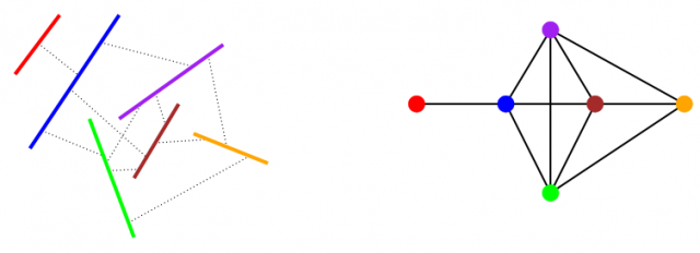
As an introduction, consider the 2D case of  disjoint line segments in the plane. Their weak visibility graph has: (1) Vertices corresponding to the segments and (2) Edges joining two vertices when the corresponding segments can be connected by a straight path which does not intersect any other segment from the original set.
Aiming to compute such a visibility graph, Pocchiola and Vegter introduced one of my favorite geometric structures, pseudo-triangulations, which allowed them to give an algorithm which runs in  time and uses
  space 3, for
  the size of the output.
Back to the Spider-Man 3D problem, the paper by Carmi et al. starts with a scene which is somehow similar to the one above. They consider vertical poles on the plane along the  -axis, for which the weak visibility graph has: (1) Vertices corresponding to poles, and (2) Edges joining two vertices when the corresponding poles are visible to each other.
For such a scenario, the authors describe an output-sensitive algorithm running in  time, for the number of edges in the output. Then, they show how to update such a data structure inserting a pole in
  time and deleting a pole in
  time.
time.
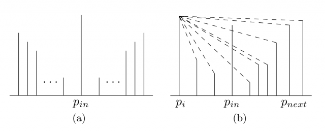
In the left picture (a) of the figure, before the insertion of the pole  every pole sees each other, so that inserting implies removing
  visibility edges. In the right picture (b), the poles between and
  are no longer visible from
  after the insertion of .
Next, Carmi et al. move to a 3D scenario with walls parallel to the  -axis, possibly with different heights.
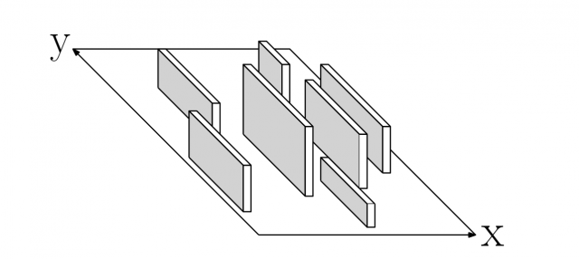
For such a scene, the authors aim to compute the horizontal weak visibility graph, which has: (1) Vertices corresponding to walls, and (2) Edges joining two vertices when there exists one point on each of the corresponding walls, both points with the same -coordinate, which can be connected by a straight path not intersecting any other wall. To begin with, a naive algorithm using the plane sweep technique (ref. 2) is presented.
In order to compute the adjacency matrix of the desired visibility graph, the algorithm sweeps the space along the -axis, with a plane parallel to the  -plane. It performs pole-insertion and pole-deletion operations when reaching, respectively, the beginning or the end of a wall. Overall, there are insertions and deletions, leading to an
  running time.
Going further, the paper proposes a more sophisticated algorithm for this parallel-walls 3D scenario. It uses fully persistent search trees 4 and achieves a running time in  .
.
Finally, the paper considers the most general case of arbitrary (vertical) walls. Given a scene of walls, possibly with different heights, based on the  -plane, the authors look for the horizontal weak visibility graph, defined as above. Their algorithm, which is similar to the sophisticated one in the previous case, except for taking into account two new types of events, runs in time.
Unfortunately, it was not Spider-Man who asked the authors to solve this problem. It actually arose during the development of a GNSS-signals simulator 5, which had to deal with the inaccuracy of GPS devices in urban regions. Usually, when such a device is located amid buildings, the signals are reaching in an indirect manner, being reflected by the walls of the buildings.
The simulator needed to compute all signal paths from the satellite to the receiver which bounce on walls at most twice. Using the visibility graph of the underlying urban region led to a significant reduction on the number of pairs of walls to be considered. In turn, this led to a dramatic improvement of the response time, allowing the simulator to perform well in real-time.
Therefore, it is you and me instead of Spider-Man who will benefit from the results by Carmi et al., which may help to palliate the inaccuracy of our navigators when we move amid buildings.
References
- Carmi P., Friedman E. & Katz M.J. (2015). Spiderman graph: Visibility in urban regions, Computational Geometry, 48 (3) 251-259. DOI: http://dx.doi.org/10.1016/j.comgeo.2014.10.004 ↩
- M. de Berg, O. Cheong, M. van Kreveld, and M. Overmars. Computational Geometry, Algorithms and Applications. Springer, 3rd edition (2008).ISBN: 978-3-540-77974-2. ↩
- M. Pocchiola and G. Vegter. Topologically sweeping visibility complexes via pseudotriangulations. Discrete and Computational Geometry, 16:4 (1996), pages 419-453. DOI: http://dx.doi.org/10.1007/BF02712876 ↩
- J.R. Driscoll, N. Sarnak, D.D. Sleator, and R.E. Tarjan. Making data structures persistent. Journal of Computer and System Sciences, 38:1 (1989), pages 86-124. DOI: http://dx.doi.org/10.1016/0022-0000(89)90034-2 ↩
- B. Ben-Moshe, P. Carmi, E. Friedman, and M.J. Katz, Modeling GNSS signals in urban canyons. Manuscript, 2012. ↩
2 comments
[…] Todos sabemos cómo se mueve Spiderman por la ciudad, disparando telas de araña de pared en pared. Pero, ¿te has preguntado alguna vez si usa realmente la ruta más corta? Y si esto es así, ¿cómo la calcula? Para […]
[…] dimentsio bat atxikitzen diotelako guzti honi. David Ordenek diosku nola konpondu arazoa Helping Spider-Man to plan his moves efficiently […]